Author: Jean-Louis Pinault (version française: ici)
This article attempts an objective approach to climatology by focusing both on the natural variability of the climate at different time scales, as well as on anthropogenic warming, especially noticeable since the early 1970s. While the natural variability of the climate finds its source mainly in the modification of the oceanic western boundary currents (such as the Gulf Stream) governed by the subtropical gyres, the anthropogenic warming, meanwhile, is based on atmospheric phenomena at altitude, involving both greenhouse gases and water vapor which plays an amplifying role.
Contents
- Attempt an objective approach to climatology
- Natural climate variability, anthropogenic impact
- Subharmonic modes
- The climate at different time scales
- The El Niño phenomenon
- What is the future of our planet?
Attempt an objective approach to climatology
Climatology is a young discipline, the essential of which remains to be discovered. The warming observed since the beginning of the industrial era is a reality, but the part attributable to human activities, to the emission of greenhouse gases in particular, is sometimes controversial. For the climate has always varied over time, which is confirmed by the archives obtained from ice or sediments cores, the first collected in the polar caps and the second in the ocean trenches. In addition, the recent evolution of the average temperature of the earth’s surface is difficult to grasp, with the required precision. The estimates made a few years ago, which showed a slowdown in global temperature growth starting from the end of the 20th century, the famous ‘hiatus’ which seemed to call into question any causal relationship between the growth of greenhouse gases and its assumed effects have been invalidated and replaced by more representative measures. The CRU (Climatic Research Unit, University of East Anglia) has made a retrospective correction by integrating more data, including the Russian Arctic, now showing a continuous increase in temperature.
These uncertainties, not to mention the images of pure communication that proved to be untrue, still fuel a certain skepticism aimed at calling into question the methodological approach of the Intergovernmental Panel on Climate Change (IPCC). Denying or minimizing by pure egocentrism or based on fallacious pseudo-scientific arguments, the anthropogenic impact on the increase of CO2 in the atmosphere as well as its climatic incidence would raise an irresponsible arrogance. Because the impact of human activities on global warming is undeniable and can now be assessed objectively thanks to recent work on the resonance of Rossby waves (baroclinic waves resulting from the oscillation of the thermocline at a depth of a hundred meters, or even more, which separates warm surface water from deeper, more dense cold water) from oceanic gyres under the effect of solar and orbital forcing. This breakthrough confirms that most of the warming observed since the 1970s is attributable to humans. The average temperature of the earth’s surface has increased by 0.8 ° C in 50 years, linearly. No inflection is perceptible, which suggests the inexorable continuation of this rise over the next decades if the production of greenhouse gases continues to increase at the frenetic pace we are currently experiencing.
This apparently low temperature rise has however an important impact on the meteorological events because of the increase in energy available to supply cyclonic and anticyclonic systems, leading to more extreme events. Nothing like this has been observed so quickly during the Holocene covering the last 12,500 years of our history.
The purpose of this article is not to make overwhelming revelations, much less to fuel new controversies. It is to reinforce the growing awareness of planetary challenges in the light of the latest scientific publications, including those of the author, and relating to climate variability in the mid- and long-term as well as the mechanisms responsible for anthropogenic impact on the current climate. Because knowledge was still lacking to unambiguously separate the natural variations of the climate from those linked to human activity.
Natural climate variability
In many cases paleoclimatology is still at the stage of speculating what may have been the underlying causes of rapid climate transitions, cycles and forcing effects. This leads us to how the climate system responds to external stimuli with its own dynamics. When the latter is consistent with an external stimulus, a resonance phenomenon occurs. The study of such resonances therefore tells us about the internal dynamics of the climate system, spearheading our understanding of the mechanisms involved in vagaries of climate.
How the solar and orbital cycles influence the surface temperature of our planet has raised many questions since the works of Milankovitch (1879-1958). Understand the vagaries of climate becomes possible from the archives of past climate. We have, in fact, over a few decades data of exceptional quality for tracing the climate up to several million years before present (BP), with a resolution of a few years. This technological feat was made possible through the analysis of stable isotopes[i] in ice cores from the Arctic and Antarctic ice caps and in sediment cores from the ocean trenches.
The analysis of ice cores plays a key role in understanding the different mechanisms involved in the natural evolution of climate over the last major cycles of glacial and interglacial periods. The oldest records obtained to date cover 800,000 years, the second half of the Quaternary.
Sediment cores allow the study of the composition of the different layers of sediment accumulated over time on the ocean floor. There are fossil microorganisms composed of calcium carbonate. By studying the « abundance ratio » of some isotopes, past climates can be reconstructed going back millions of years, as well as how the oceans have evolved in different climatic periods (temperature, salinity, nutrients,…).
Our wanderings as to the mechanisms controlling climate variability result from the fact that research has mainly focused on atmospheric and terrestrial phenomena in recent decades, whether they refer to human activities or to solar cycles. One example is the work on the Greenland inlandsis to explain the climatic response to orbital cycles. It takes ingenuity to imagine this glacier unstable enough to slide and then recover at the whim of small variations in the solar irradiance subjected to different orbital cycles.
This article attempts to provide some answers by invoking a previously unknown phenomenon, which is the resonance of Rossby waves winding around the 5 subtropical ocean gyres. The Rossby waves of periods 1/2, 1, 4 and 8 years give rise to the rainfall oscillation phenomenon that is sometimes confused with El Niño. The regions affected can undergo a succession of dry and then wet years as is the case in Western Europe.
On the Rossby waves of short periods are superimposed waves of long periods. Like short-period waves, they originate where the western boundary currents move away from the continents and then leave the gyre beyond half a wavelength towards the poles. This concept being supported both by the observation of long-term thermal anomalies around the North Atlantic gyre as well as by the resolution of the equations of motion of long-wavelength Rossby waves, it turns out that the driver of climate change is oceanic, the atmosphere playing only the role of vector between the oceans and the continents, like the El Niño phenomenon. Ocean gyres enter into resonance with the solar and orbital cycles, storing heat or on the contrary restoring it: the resonance of gyral Rossby waves tightly conditions the energy balances of our planet, mediating between solar and orbital forcing and climate impact.

Subharmonic modes
Subharmonic modes provide physical bases for resonant phenomena that many researchers have foreseen for a long time to explain how the efficiency of solar and orbital forcing could vary by a factor of 5, even more, during glacial-interglacial periods, as well as the contribution of the natural variability in the global climate change that prevailed since the beginning of the 20th century.
The equations of motion of gyral Rossby waves give them amazing properties. Half a wavelength of long period gyral Rossby waves wind around each of the 5 subtropical gyres, forming several turns while propagating cyclonically. They overlap with the wind-driven current of the gyre which is driven by westerly winds at mid-latitudes and by trade winds at low latitudes. Gyral Rossby waves do not dampen as their period increases. Being forced resonantly by the solar and orbital cycles, the Rayleigh friction of these waves is compensated by the extension of the duration of the forcing when the period increases.
Several gyral Rossby waves of different periods overlap. Sharing the same current of the gyre, they are coupled. Like any system of resonantly forced coupled oscillators, these waves oscillate in subharmonic modes, which means that their periods are multiples of the period of the fundamental wave which is here annual due to the declination of the sun. The average periods of the main modes observed are (in years) 1, 4, 8 = 4 × 2, 64 = 8 × 8, 128 = 64 × 2 (solar forcing, Gleissberg cycle), 256 = 128 × 2, 768 = 256 × 3 (solar forcing), 24576 = 768 × 32 (orbital forcing, precession), 49152 = 24576 × 2 (orbital forcing, obliquity), 98304 = 49152 × 2 (orbital forcing, eccentricity). The forcing efficiency is all the higher as its period is closer to one of the resonance periods of the wave. Each subharmonic mode corresponds to an integer number of turns that propagate around the gyre before leaving it to move towards one of the poles. For the 128-year period the wave travels 2 turns in the North and South Atlantic, 1 turn in the North and South Pacific and 3/2 turns in the South of the Indian Ocean.
Oceanic Rossby waves impact the climate due to the sea surface temperature anomalies they generate, which can cause atmospheric baroclinic instabilities. Long-period Rossby waves play a special role because of the powerful positive feedback they exert on western boundary currents whose speed is strongly impacted by solar and orbital forcing. Indeed, the modulated polar current of the Rossby wave, which is proportional and in phase with the oscillation of the thermocline, is superimposed on the wind-driven current of the gyre.
The climate at different time scales
Thus, the modulated response of subtropical gyres helps explain, through observations and based on irrefutable physical basis, climate change at different time scales. The amplifying effect of solar and orbital forcing comes from the positive feedback exerted by the geostrophic current (resulting from the combination of gravity and inertial forces due to the rotation of the earth) of the gyral Rossby wave: the oscillation of the thermocline is amplified by the geostrophic current which warms or cools, as the western boundary current accelerates or slows down. This occurs according to the same subharmonic modes as the subtropical gyres. Based on this new phenomenon, this article discusses climate variability with fresh eyes while solving some puzzles on ocean circulation.
The Holocene
The climate during Holocene, which began with the interglacial period about 12500 years ago, can be studied from proxies of solar irradiance and Earth’s average temperature in both hemispheres. From the coupling between solar irradiance and global mean temperature is deduced information about the internal dynamics of the climate system. Furthermore, superimposed on oscillations are several distinct climate steps. Climatic variations occur essentially in two subharmonic modes of average periods 768 and 128 years. Their study covers the frequency bands 576-1152 years and 96-192 years, respectively.
With regard to the cycle of 768-year average period, the amplitude of the forcing efficiency, that is to say the sensitivity of the global temperature (°C) to solar insolation (W/m2), varies greatly during the Holocene, progressively increasing from 1.5 °C×(W/m2)-1 to 0.5 °C×(W/m2)-1 and this in the two hemispheres. The large thermal amplitude observed at the beginning of the Holocene reflects the advance of the pack ice: the thermal gradient between the mid- and low-latitude of the gyres is maximum, which strengthens the oscillation of the thermocline and, therefore, the polar modulated current of the gyres, from which follows the acceleration / deceleration of the western boundary currents. Little ice ages can be observed during the cooling phase of the cycle when the current of the gyre at high latitudes, cold and salty, plunges under the less dense surface layer. The heat exchanges between the western boundary currents and the continents cease during the complete duration of inversion of the surface ocean layers. This results in an abrupt cooling phenomenon due to reduced heat fluxes between the low and high latitudes of the gyres.
While the 768-year period cycle is a pure harmonic of longer period cycles impacted by orbital cycles, the 128-year period cycle is, at least in part, forced by the Gleissberg cycle of the sun. The efficiency of forcing varies widely during the Holocene, weakening considerably during periods of low solar activity.
The glacial-interglacial period
As for the Holocene, the comparative study of the global average temperature and the solar irradiance (which is here calculated from Milankovitch parameters and no longer observed from proxies) can be carried out in order to deduce the efficiency of orbital forcing. The global mean temperature is deduced from the records in ice and sediment cores. Due to the resonant nature of the climate system, forcing is all the more efficient as its period is closer to one of the resonance periods. During the ice-interglacial era, climatic variations mainly occur in three frequency bands corresponding to the three orbital parameters which are eccentricity, precession, and obliquity.
The forcing efficiency in the 73.7–147.5 Ka band (cycle of 98.3 Ka period) increases from around 1.4 Ma, going from 0.7 to 5.0 °C×(W/m2)-1, which confirms that the forcing period due to the eccentricity approaches the resonance period over time (this phenomenon can be observed from the time / frequency representation of the orbital variation of the insolation). Above 1.4 Ma the dominant period was 49.2 Ka due to the obliquity whose period is 41 Ka, until the period of forcing due to eccentricity, whose period is about 100 Ka, is close enough to the resonance period to prevail. This is what gave rise to the mid-Pleistocene transition.
During the last 0.8 Ma the forcing efficiency in the bands 36.9-73.7 Ka (cycle of 49.2 Ka period) and 18.4-36.9 Ka (cycle of 24.6 Ka period characteristic of the precession whose period is around 23.5 Ka) varies around a value close to 1 °C×(W/m2)-1. The transitions reflect the movements of the gyres’ centroids which more or less favor the tuning between the forcing and resonance periods.
The current climate
With regard to the anthropogenic impact, research focuses mainly on the mechanisms of amplification of the greenhouse effect. The cumulative effect of greenhouse gases on surface temperature cannot explain the variations in the observed average temperature, the anthropogenic component of which has increased linearly since the 1970s. This supposes a powerful positive feedback of the greenhouse effect on the global temperature.
The share of natural variations in the earth’s surface temperature can now be estimated with precision from thermal anomalies observed on each of the 5 subtropical ocean gyres. These start a decrease (a few tens of degrees) mainly due to the harmonic of 64-year average period, but which remains weak compared to the anthropic component and cannot be enough to reverse the trend.
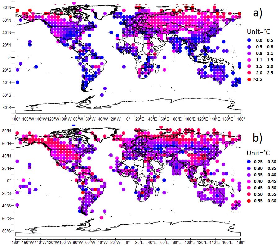
Under these conditions, considering the natural component of the surface temperature makes it possible to know precisely the anthropogenic component obtained by subtracting the natural component from the surface temperature measured from terrestrial meteorological stations or from satellites. This exercise
The spatial distribution of the anthropogenic impact on the climate, which varies according to latitude, but also to longitude, then highlights the mechanisms responsible for the amplifying effect of water vapor on the warming induced by greenhouse gases according to different climatic regimes. The correlation of the increase in temperature of anthropogenic origin with the spatial distribution of the amplitude and the phase of the precipitation height in two bands of periods, 8-16 months, and 5-10 years, specifies the mechanisms involved.
The frequency representation of the reduced precipitation heights (divided by the average rainfall height) reveals two very distinct rainfall regimes depending on whether they have an annual or multi-annual periodicity. In the first case, low pressure systems occur especially at the end of summer when the temperature difference between the surface and the upper layers of the troposphere is maximum while in regions with multi-year precipitation regimes cyclonic systems result in sea surface temperature anomalies produced by Rossby waves at high latitudes of the 5 subtropical gyres. However, the first regions are more impacted than the second, which suggests the determining role of the adiabatic lapse rate (the way in which the temperature of the atmosphere varies with altitude) in the amplification phenomenon.
The latitudinal and longitudinal variation of the anthropogenic response is explained from the physical properties of moist adiabat (the lapse rate in the presence of water vapor) and, with it, the emission of thermal radiation from the water vapor at an altitude close to 4.3 km (at mid-latitudes). It is in fact at this altitude that the thermal radiation emitted from the surface of the earth, whose wavelength lies in the saturated absorption band of water vapor, escapes to space. These thermal photons diffuse in the layer of the atmosphere which is opaque to them until they escape where the atmosphere becomes transparent.
As a result of readjustment of the moist adiabat, the increase in surface temperature raises the layer from which diffuse photons are emitted, which has the effect of cooling it and thus reducing the thermal radiation which escapes towards space. Warming of the atmosphere follows and hence of the surface of the earth. This results in a powerful positive feedback since any heating of the atmosphere, however small, induces processes which tend to amplify it. The physical phenomena involved are robust because the atmospheric layer from which thermal photons are emitted can be assimilated to a black body. In other words, the thermal radiation that escapes depends only on the temperature of the layer, whether the water is in the vapor state or condensed to form clouds.
One of the most important consequences of global warming is melting the polar ice. This phenomenon is followed with the greatest attention due to the acceleration of the phenomena. Satellite measurement of sea ice concentration by microwave provides real-time information.

In particular, Arctic amplification, which occurs mainly at the end of the summer, involves the moist adiabat. It approaches the dry adiabat due to the low temperatures of the upper atmosphere. However, the Antarctic is less sensitive to anthropogenic impact because the upper atmosphere remains dry there in all seasons, which means that the adiabatic lapse rate can be assimilated to a dry adiabat which is invariable (the reduction of albedo due to the melting of the ice only partially contributes to the feedback).
Another consequence of global warming is the increase in extreme events. At mid-latitudes, they are the Marine Heatwaves (MHWs) and the subtropical cyclones. The analysis of the different stages leading to subtropical low-pressure systems makes it possible to address an essential problem that relates to the presumed impact of anthropogenic forcing. One mechanism for the increase in such transient events discussed in the literature is related to the slowing of the predominant westerly wind circulation evident in observational data, due to a strong warming of the Arctic as a result of global warming. Such a slowdown has been linked to observed increases in the persistence of weather systems.
By influencing the rapid cycles of cyclogenesis, such a mechanism could contribute to explaining the increase in the frequency of extreme rainfall events observed during the last decades in the northern hemisphere, in particular in the North America. But the ubiquity of the increase in the frequency as well as the intensity of extreme rainfall events also suggest an evolution in the mechanisms favoring the development of cyclonic flows at the synoptic scale. This hypothesis is corroborated by the fact that extreme rainfall events occur in places deemed not to be flood-prone, causing numerous victims, as happened in Germany in July 2021, thus deceiving the vigilance of weather-watch systems.
As shown in a recent article, the development of coherent SST anomalies, the main driver of synoptic-scale subtropical cyclones, is unambiguously linked to the propagation of oceanic Rossby waves. These result from solar forcing, independent of anthropogenic forcing. In contrast, other mechanisms related to global warming appear to be decisive in the context of slow cycles during which the coalescence of low-pressure systems occurs. Such mechanisms are strengthened by a temperature increase of ocean surface water associated with an overall increase in atmospheric humidity, which lowers the dew point and favors the formation of fronts. In return, the extension of the low-pressure system at the synoptic scale centered on a continental low favors the feeding of the cyclonic flow by overlapping over surrounding Sea Surface Temperature anomalies. Owing to the accumulated latent heat, with regard to their internal energy these low-pressure systems promote upper-level lows, favoring blocks. This may explain the record precipitations observed during the last decades when pouring over regions deemed not to be flood prone, as has occurred in many places in Western and Central Europe.
The El Niño phenomenon
It is the result of the coupling of two quasi-stationary Rossby waves in the tropical Pacific Ocean, whose average period is respectively annual and quadrennial. The annual wave is forced by the trade winds. The quasi-stationary quadrennial wave forms two main antinodes in phase opposition, the western antinode formed of off-equatorial Rossby waves and the central-eastern antinode, result of the superposition of a Rossby wave and a Kelvin wave, both trapped by the equator but propagating in opposite directions.

Let us note that this seesaw movement between a western antinode formed of off-equatorial Rossby waves and a central-eastern antinode where a Rossby wave and a Kelvin wave, both equatorial, are superimposed, is observed in the three tropical oceans. In the Atlantic Ocean its period is annual while in the Indian Ocean it is biennial. In any case, the movement of warm water induces a climate response.
The quadrennial wave generates an El Niño event at the end of its eastward phase propagation, the merging of warm waters from the western Pacific and cold waters of the eastern Pacific stimulating evaporation processes. ENSO (El Niño Southern Oscillation) has a major climatic impact by producing a noticeable warming phenomenon at mid or even high latitudes for a few months. Its average period is 4 years, but it undergoes a strong variability which reflects the specific dynamics of the quadrennial wave. ENSO may occur in the central or eastern Pacific depending on the expected date of occurrence compared to a regular 4-year cycle. It can be followed by La Niña during the recession of the quadrennial wave to the west when it stimulates upwelling of deep cold waters off the Peruvian and Chilean coasts.
At longitude 180 ° W, that is to say at the most westerly point of the central-eastern equatorial antinode, subsurface water temperature anomalies precede of 8-7 months the maturation phase of ENSO. Thanks to the network of anchored probes immersed in the first hundreds of meters of the tropical Pacific it is therefore possible to predict ENSO events by simply observing the temperature of seawater where the thermocline oscillates. The date of occurrence of the anomaly and its amplitude make it possible to specify the type and intensity of the El Niño event being forming.
The intensity of ENSO varied widely during the Holocene, weakening, and then recovering. This suggests a strong interaction with the north-equatorial and south-equatorial current of the North- and South-Pacific subtropical gyres.
What is the future of our planet?
The linear growth, attributable to human activities, of the surface temperature observed since 1970 being of the order of 0.8 to 1 ° C, everything suggests that the average temperature will further increase by almost 1 ° C during the next 50 years if the increase in greenhouse gas production does not weaken. Under these conditions, the global temperature increase of 1.5 ° C set by the Paris agreements would be reached in 2045.
Despite the efforts of the IPCC, huge uncertainties remain regarding the forecasts of climate change at the regional scale, according to the different scenarios relating to the evolution of greenhouse gas emissions, but also because of the weakness of mid- and long-term climate models. But the trends we are currently seeing can only continue, if not worsen. There is no doubt that humanity will have to adapt while drastically reducing its combustion gas emissions by speeding up the ecological transition.
I praise the sagacity and the clairvoyance of climatologists who put forward the hypothesis of anthropogenic warming from the 80s. The precursor works of Arrhenius were of no use since the required physical bases were not yet established at the end of the 19th century. Little was known about the feedback mechanisms, which precluded any quantitative approach to the evolution of mean surface temperature. Numerous forces have protested against what may have seemed intuitive, even misleading, and fundamentally called into question the evolution of our society. Over 30 years have passed, and climate science has made a tremendous leap, confirming, and specifying the premonitions.
References
Arrhenius, S. (1896) On the Influence of Carbonic Acid in the Air upon the Temperature of the Ground, Philosophical Magazine and Journal of Science, 5, 41, 237-276.
Augustin, L., Barbante, C., Barnes, P.R.F., Barnola, J.M., Bigler, M., Castellano, E., Cattani, O., Chappellaz, J., Dahl-Jensen, D., Delmonte, B., Dreyfus, G., Durand, G., Falourd, S., Fischer, H., Fluckiger, J., Hansson, M.E., Huybrechts, P., Jugie, G., Johnsen, S.J., Jouzel, J., Kaufmann, P., Kipfstuhl, J., Lambert, F., Lipenkov, V.Y., Littot, G.C., Longinelli, A., Lorrain, R., Maggi, V., Masson-Delmotte, V., Miller, H., Mulvaney, R., Oerlemans, J., Oerter, H., Orombelli, G., Parrenin, F., Peel, D.A., Petit, J.-R., Raynaud, D., Ritz, C., Ruth, U., Schwander, J., Siegenthaler, U., Souchez, R., Stauffer, B., Steffensen, J.P., Stenni, B., Stocker, T.F., Tabacco, I.E., Udisti, R., van de Wal, R.S.W., van den Broeke, M., Weiss, J., Wilhelms, F., Winther, J.-G., Wolff, E.W., and Zucchelli, M. (2004) Eight glacial cycles from an Antarctic ice core. Nature 429: 623–628.
Berger, A., 1992, Orbital Variations and Insolation Database. IGBP PAGES/World Data Center for Paleoclimatology Data Contribution Series # 92-007. NOAA/NGDC Paleoclimatology Program, Boulder CO, USA.
Bianchi, G.G. and I.N. McCave, (1999) Holocene periodicity in North Atlantic climate and deep-ocean flow south of Iceland, Nature, 397,515-513.
Bond, G., H. Heinrich, W. Broecker, L. Labeyrie, J. Mcmanus, J. Andrews, S. Huon, R. Jantschik, S. Clasen, C. Simet (1992), « Evidence for massive discharges of icebergs into the North Atlantic ocean during the last glacial period ». Nature 360 (6401): 245–249. doi:10.1038/360245a0
Bond, G., W. Showers, M. Cheseby, R. Lotti, P. Almasi, P. deMenocal, P. Priore, H. Cullen, I. Hajdas and G. Bonani, (1997) A pervasive millenial-scale cycle in North Atlantic Holocene and glacial climates. Science, 278, 1257-1265.
Bond, G., Kromer, B., Beer, J., Muscheler, R., Evans, M.N., Showers, W., Hoffmann, S., Lotti-Bond, R., Hajdas, I., and Bonani, G. (2001) Persistent solar influence on North Atlantic climate during the Holocene. Science 294: 2130–2136.
Chambers, F.M., Ogle, M.I., and Blackford, J.J. (1999) Palaeoenvironmental evidence for solar forcing of Holocene climate: linkages to solar science. Progress in Physical Geography 23: 181–204.
Dansgaard W., Johnsen S. J., Møller J., Langway Jr C. C. (1969) One Thousand Centuries of Climatic Record from Camp Century on the Greenland Ice Sheet, Science, 166, 3903, 377-380, DOI: 10.1126/science.166.3903.377
Dansgaard, W., S.J. Johnson, H.B. Clausen, D. Dahl-Jensen, N.S. Gundenstrup, C.U. Hammer, C.S. Hvidberg, J.P. Steffensen, A.E. Sveinbjornsdottir, J. Jouzel, G. Bond (1993) Evidence for general instability of past climate from a 250-kyr ice-core record. Nature, 364, 218-220.
Ganopolski, A., and S. Rahmstorf (2001) Rapid changes of glacial climate simulated in a coupled climate model, Nature, 409, 153– 158.
Gavin, D. G., Henderson, A. C. G., Westover, K. S., Fritz, S. C., Walker, I. R., Leng M. J., and Hu, F.S. (2011) Abrupt Holocene climate change and potential response to solar forcing in western Canada. Quaternary Science Reviews 30: 1243–1255.
Giraudeau, J., M. Cremer, S. Mantthe, L. Labeyrie, G. Bond (2000) Coccolith evidence for instability in surface circulation south of Iceland during Holocene times. Earth and Planetary Science Letters, 179, 257-268.
Grootes, P.M., and M. Stuiver (1997) Oxygen 18/16 variability in Greenland snow and ice with 10^3 to 10^5-year time resolution. Journal of Geophysical Research 102:26455-26470. ftp://ftp.ncdc.noaa.gov/pub/data/paleo/icecore/greenland/summit/gisp2/isotopes/gispd18o.txt
Jones, P. D., D. H. Lister, T. J. Osborn, C. Harpham, M. Salmon, and C. P. Morice (2012), Hemispheric and large-scale land surface air temperature variations: An extensive revision and an update to 2010, J. Geophys. Res., 117, D05127, doi:10.1029/2011JD017139, https://crudata.uea.ac.uk/cru/data/temperature/CRUTEM4-gl.dat
Jouzel, J., L. Merlivat (1984) Deuterium and oxygen 18 in precipitation: Modeling of the isotopic effects during snow formation, Journal of Geophysical Research: Atmospheres, 89, D7, 11749–11757
Jouzel, J., C. Lorius, J. R. Petit, C. Genthon, N. I. Barkov, V. M. Kotlyakov and V. M. Petrov (1987) Vostok ice core: a continuous isotope temperature record over the last climatic cycle (160,000 years), Nature, 329, 402-408.
Jouzel, J., V. Masson-Delmotte, O. Cattani, G. Dreyfus, S. Falourd, G. Hoffmann, B. Minster, J. Nouet, J.M. Barnola, J. Chappellaz, H. Fischer, J.C. Gallet, S. Johnsen, M. Leuenberger, L. Loulergue, D. Luethi, H. Oerter, F. Parrenin, G. Raisbeck, D. Raynaud, A. Schilt, J. Schwander, E. Selmo, R. Souchez, R. Spahni, B. Stauffer, J.P. Steffensen, B. Stenni, T.F. Stocker, J.L. Tison, M. Werner, and E.W. Wolff. (2007) Orbital and Millennial Antarctic Climate Variability over the Past 800,000 Years. Science, Vol. 317, No. 5839, pp.793-797, 10 August 2007 ftp://ftp.ncdc.noaa.gov/pub/data/paleo/icecore/antarctica/epica_domec/ edc3deuttemp 2007.txt
Kao H.Y. and Yu J.Y. (2009) Contrasting Eastern-Pacific and Central-Pacific types of ENSO, J. Climate, 22 (3), 615–632, doi: 10.1175/2008JCLI2309.1
Karlén, W. and Kuylenstierna, J. (1996) On solar forcing of Holocene climate: evidence from Scandinavia. The Holocene 6: 359–365.
Lisiecki, L.E. and Raymo M.E. (2005) LR04 Global Pliocene-Pleistocene Benthic d18O Stack. IGBP PAGES/World Data Center for Paleoclimatology Data Contribution Series #2005-008. NOAA/NGDC Paleoclimatology Program, Boulder CO, USA.
Magny, M. (1993) Solar influences on Holocene climatic changes illustrated by correlations between past lake-level fluctuations and the atmospheric 14C record. Quaternary Research 40: 1–9.
Manabe R. and Wetherald R.T. (1967) Thermal Equilibrium of the Atmosphere with a given distribution of Relative Humidity, Journal of the Atmospheric Science, 24, 3
Maslin, M., D. Seidov, J. Lowe (2001). « Synthesis of the nature and causes of rapid climate transitions during the Quaternary”. Geophysical Monograph 126: 9–52. doi:10.1029/GM126p0009
de Menocal, P., J. Ortiz, T. Guilderson and M. Sarnthein (2000) Coherent High- and Low- latitude climate variability during the Holocene warm period. Science, 288, 2198-2202.
North Greenland Ice Core Project members. 2004. High-resolution record of Northern Hemisphere climate extending into the last interglacial period. Nature, v.431, No. 7005, pp. 147-151, 9 September 2004. ftp://ftp.ncdc.noaa.gov/pub/data/paleo/icecore/greenland/ summit/ngrip/isotopes/ngrip-d18o-50yr.txt
O’Brien, S. R., A. Mayewski, L.D. Meeker, D.A. Meese, M.S. Twickler, and S.I. Whitlow (1996) Complexity of Holocene climate as reconstructed from a Greenland ice core. Science, 270, 1962-1964.
Petit, J.R., J. Jouzel, D. Raynaud, N.I. Barkov, J.-M. Barnola, I. Basile, M. Benders, J. Chappellaz, M. Davis, G. Delayque, M. Delmotte, V.M. Kotlyakov, M. Legrand, V.Y. Lipenkov, C. Lorius, L. Pépin, C. Ritz, E. Saltzman, and M. Stievenard. (1999) Climate and atmospheric history of the past 420,000 years from the Vostok ice core, Antarctica. Nature 399: 429-436.
Pinault J-L (2012) Global warming and rainfall oscillation in the 5–10 yr band in Western Europe and Eastern North America, Climatic Change, Springer, vol. 114(3), pages 621-650, DOI 10.1007/s10584-012-0432-6
Pinault J-L (2013) Long Wave Resonance in Tropical Oceans and Implications on Climate: the Atlantic Ocean, Pure Appl. Geophys. 170, 1913–1930 DOI 10.1007/s00024-012-0635-9
Pinault J-L (2015) Long Wave Resonance in Tropical Oceans and Implications on Climate: The Pacific Ocean, Pure Appl. Geophys. DOI 10.1007/s00024-015-1212-9
Pinault J-L (2016) Anticipation of ENSO: what teach us the resonantly forced baroclinic waves, Geophysical & Astrophysical Fluid Dynamics, 110:6, 518-528, DOI: 10.1080/03091929.2016.1236196
Pinault J-L (2018b) The Anticipation of the ENSO: What Resonantly Forced Baroclinic Waves Can Teach Us (Part II), J. Mar. Sci. Eng., 6, 63; doi:10.3390/jmse6020063
Pinault J-L (2018a) Regions Subject to Rainfall Oscillation in the 5–10 Year Band, Climate, 6, 2; doi:10.3390/cli6010002
Pinault J-L (2018c) Resonantly Forced Baroclinic Waves in the Oceans: Subharmonic Modes, J. Mar. Sci. Eng., 6, 78; doi:10.3390/jmse6030078
Pinault J-L (2018d) Modulated Response of Subtropical Gyres: Positive Feedback Loop, Subharmonic Modes, Resonant Solar and Orbital Forcing, J. Mar. Sci. Eng., 6, 107; doi.org/10.3390/jmse6030107
Pinault J-L (2018e) Anthropogenic and Natural Radiative Forcing: Positive Feedbacks, J. Mar. Sci. Eng., 6, 146; doi:10.3390/jmse6040146
Pinault J-L (2019) Resonance of baroclinic waves in the tropical oceans: The Indian Ocean and the far western Pacific, Dynamics of Atmospheres and Oceans, Volume 89, March 2020, 101119, DOI: 10.1016/j.dynatmoce.2019.101119
Pinault J-L (2020a) Resonant Forcing of the Climate System in Subharmonic Modes, J. Mar. Sci. Eng., 8, 60; doi:10.3390/jmse8010060
Pinault J-L (2020b) The Moist Adiabat, Key of the Climate Response to Anthropogenic Forcing, Climate 2020, 8, 45; doi:10.3390/cli8030045
Pinault, J.-L. (2021a) Resonantly Forced Baroclinic Waves in the Oceans: A New Approach to Climate Variability. J. Mar. Sci. Eng. 2021, 9(1), 13; https://doi.org/10.3390/jmse9010013
Polyakov I. V., Timokhov L. A. and Alexeev V. A. (2010) J. Physical Oceanography 40, 2743
Polyakov I. V., Pnyushkov A. V. and Timokhov L. A. (2012) J. Climate 25, 8362
Schönwiese C-D; Bayer D. (1995) Some statistical aspects of anthropogenic and natural forced global temperature change, Atmósfera, 8 (1)
Steinhilber, F., et al. (2012) 9400 Year Cosmogenic Isotope Data and Solar Activity Reconstruction. IGBP PAGES/World Data Center for Paleoclimatology Data Contribution Series # 2012-040. NOAA/NCDC Paleoclimatology Program, Boulder CO, USA. ftp://ftp.ncdc.noaa.gov/ pub/data/paleo/climate_forcing/ solar_variability/steinhilber2012.txt
Taylor, K.C, R.B. Alley, G.A. Doyle, P.M. Grootes, P.A. Mayewski, G.W. Lamorey, J.W.C. White, and L.K. Barlow (1993) The ‘flickering switch’ of late Pleistocene climate change. Nature, 361, 432-436.
Willeit,M., A. Ganopolski, R. Calov and V. Brovkin, Mid-Pleistocene transition in glacial cycles explained by declining CO2 and regolith removal, Science Advances 03 Apr 2019, DOI: 10.1126/sciadv.aav7337