The current climate is the subject of intense debate because of the economic and societal implications of global warming. Greenhouse gases, mainly carbon dioxide but also other gases that are rarer but have a high absorption capacity of long-wave radiation re-emitted by the Earth, are accused of playing an important role in anthropogenic climate change. However, the actual anthropogenic impact on global temperature is poorly understood due to feedback loops and non-linear effects.

Here, we focus on natural cycles as well as the anthropogenic component of surface temperature. The latter is deduced from the instrumental surface temperature at which the natural component taken from observations of the surface of the oceans at very specific locations in the 5 subtropical oceanic gyres is subtracted. The main feedback responsible for amplifying effects is deduced from the latitudinal and longitudinal distribution of the response of the surface temperature to anthropogenic forcing, which involves the different types of climates (Pinault, 2018e).

Contents

• Natural climatic cycles
• Spatial pattern of anthropogenic and natural temperature responses
• Regions subject to rainfall oscillation in the band 5-10 years
• Regions subject to an annual precipitation regime
• Level of emission of outgoing longwave radiation in the saturated absorption bands of water vapor
• The moist adiabat
• Latitudinal variations of climate response to anthropogenic forcing
• Longitudinal variations of the climate response to anthropogenic forcing
• Anthropogenic forcing in a nutshell

Natural climatic cycles

As we will see, if we ignore at first the anthropogenic impact on the climate, the natural variability of the surface temperature of the continents can be deduced from the variability of certain anomalies of the surface temperature of the oceans representative of thermal exchanges between oceans and continents. The ocean contribution to global temperature is obtained from a linear combination of these sea surface temperature (SST) anomalies. The oceanic contribution in the global temperature can be formally identified after 1870, the date from which the data is available, and before the anthropogenic impact becomes noticeable.

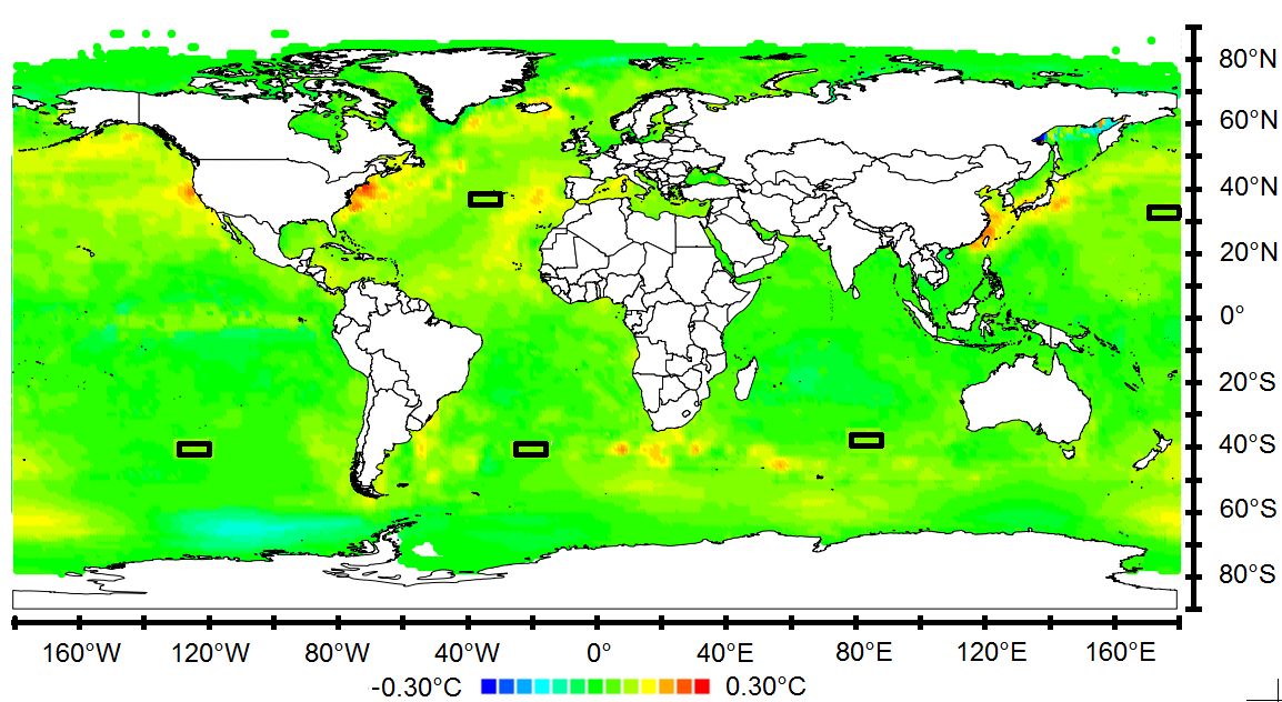
The impact on climate of the sea surface perturbation ΔT, which reflects the persistence of the vertical thermal gradient, either reinforces or, on the contrary, reduces evaporation. This results from atmospheric baroclinic instabilities that may lead to the formation of cyclonic systems. Because baroclinic instabilities of the atmosphere are most active when the resulting synoptic-scale eddies are stimulated and guided by the subtropical jet streams, SST anomalies are located at high latitudes of the gyres around 40°. They have to be representative of long-period Gyral Rossby waves (GRWs), which correspond to high subharmonic modes, to accurately reflect the persistence of their continental replicas.

Consequently, areas representative of the oceanic signature in the global temperature are to be selected at high latitudes of the five subtropical gyres. The perturbation ΔT represented by the SST anomalies, averaged over each area, is deduced from the land surface temperature. The resulting oceanic signature of the global temperature is obtained by doing the weighted average of the SST anomalies in the five subtropical gyres. The weights are indicative of the incidence on the global temperature of the corresponding gyres, that is, they are approximately proportional to the areas of the continents impacted by each of the gyres.

Some continental regions are directly impacted by heat exchanges between the oceans and the continents. To these continental regions can be associated particular SST anomalies by jointly analyzing, both in space and time, the SST and the rainfall oscillations in the 5–10 year band. This method allows representing the inland areas subject to such rainfall oscillation, from which the signatures of the SST and rainfall height anomalies can be unambiguously associated. This is made possible because of the selectivity of both SST and rainfall height anomalies within this band. The active SST anomalies are located on the internal antinodes of the GRWs (where the thermocline oscillates) for the relevant subharmonic modes. The main areas subject to rainfall oscillation at mid-latitudes where condensation / precipitation of water vapor releases the latent heat, are Southwest North America, Texas, Southeastern and Northeastern North America, Southern Greenland, Central and Western Europe and Western Asia, the region of the Río de la Plata, Southwestern and Southeastern Australia, and Southeast Asia.

However, SST anomalies in the 5–10 year band are representative of short-term exchanges between the oceans and the continents resulting from the resonance of GRWs for low subharmonic modes and their inland thermal imprints are evanescent. For these reasons, representative areas of SST anomalies on the long-period internal antinodes, which correspond to higher subharmonic modes, must be judiciously selected to accurately represent the persistence of continental thermal footprints. Accuracy of the SST anomalies averaged over such areas requires the latter are as small as possible not to integrate short-term exchanges the signature of which is masked by long-term exchanges. Short-term and long-term exchanges are governed by short-wavelength and long-wavelength GRWs, respectively. Internal antinodes of short-wavelength GRWs extend from where the western boundary current leaves the coast to the bifurcation of the re-circulating wind-driven current of the gyre and the drift current leaving the gyre. Internal antinodes of long-wavelength GRWs extend all around the gyres so that areas representative of persistent exchanges are necessarily located to the east of the short-period internal antinodes.

Preselected areas are considered as representative of thermal exchanges in the perturbed state of the global climate system when the oceanic perturbation ΔT, that is, the weighted average of SST anomalies over the five subtropical gyres, is a replica of the instrumental global temperature. This can be done before the global temperature is subject to anthropogenic warming. Then, the net anthropogenic contribution in the global temperature can be estimated by subtracting from the latter the weighted sum of the SST anomalies from the global temperature. Actually, the contributions of the SST anomalies are estimated by using the least squares method, that is, by minimizing the sum of the squares of the differences between the instrumental global temperature and the weighted sum of the SST anomalies within a relevant interval of time, the sum of the weighting factors being one.

Oceanic signatures exhibit particular behaviors according to the gyres. In the Figure the instrumental surface temperature is compared to the weighted sum of SST anomalies w_NANA+w_NPNP+w_SASA+w_SPSP+w_SISI where the weighting factors are w_NA=0.50, w_NP=0.17, w_SA=0.15, w_SP=0.13, w_SI=0.05. Systematic differences are observed. Beyond 1970, the discrepancies highlight the contribution of the anthropogenic warming. Before 1900 they reflect systematic errors on measurements.

The contribution of the natural component in the band 48-96 years, whose amplitude of variation is 0.3°C, is significant as well as that in the band 192-576 years, which varies between ±0.1°C. In the band 96-192 years it is associated with the Gleissberg solar cycle.

Spatial pattern of anthropogenic and natural temperature responses (Pinault, 2018e)

The weights associated with the SST anomalies that represent at best the gridded surface temperatures Ts are estimated by using the same least squares method as that explained previously. Here, the time interval from which the fitting is performed is 1940-1970, for which the weights are the most precise and the most representative of natural forcing when the surface temperatures are considered individually in the 5°×5° grid. This choice allows us to minimize the noise in the spatial pattern of the natural temperature. However the estimation of the part of the anthropogenic response within Ts by subtracting from the latter the weighted sum of the SST anomalies very little depends on the time interval, 1900-1970 or 1940-1970.

The temperature response to the natural radiative forcing exhibits a low spatial variability in both hemispheres. In the northern hemisphere it is because the temperature response of the Atlantic and the Pacific oceans in 2015 are close (the temperature increase since 1970 in the Pacific is slightly lower than in the Atlantic). The influence of the Pacific can be seen in the Central Asia whereas North America and Europe are rather influenced by the Atlantic. The southern hemisphere reflects the influence of the warmer Indian Ocean than the other two oceans. Everywhere the natural temperature response is positive because all oceanic signatures increase since 1970s. The increase is most noticeable in the North America and north of 60°N, where it reaches 0.6 ° C.

In addition to the natural response, the part of the anthropogenic response within the instrumental surface temperature Ts shows considerable spatial variability. Lower than 0.8°C and even 0.5°C in Australia, southern South America, eastern North America, northern and Western Europe, and Southeast Asia it overreaches 2°C in Eastern Europe, Russia, Kazakhstan, Mongolia, east of North America, east of Brazil, eastern Africa, Angola, Namibia, even more than 2.5°C north of 70°N. This great disparity questions the nature of the positive feedback loop responsible for such amplification in some regions, presenting both latitudinal and longitudinal variability.

Regions subject to rainfall oscillation in the band 5-10 years 

The distribution of extra-tropical regions with low anthropogenic impact coincides with those subject to the rainfall oscillation in the 5-10 year band. In the North American continent, these are mainly the regions of eastern and south-western United States. In South America this concerns the countries of the north, and both eastern and southern Argentina. In Europe, these are the South Greenland, and western and northern countries. In Africa, the oscillation concerns the North of the Maghreb countries and South Africa. In Oceania the oscillation is observable almost everywhere.

At mid-latitudes, rainfall oscillation in the 5-10 year band characterizes regions with a strong oceanic influence. In other words, the cyclonic systems that traverse these regions have an oceanic origin. In the equatorial belt, rainfall oscillation results from atmospheric Rossby and Kelvin waves. These regions are little impacted by anthropogenic forcing.

Regions subject to an annual precipitation regime

Areas that are subject to high latitudinal variability of anthropogenic forcing are characterized by a high amplitude of the rainfall oscillation in the 0.5-1.5 year band, exhibiting a strong seasonality. The annual rainfall pattern displays a peak time in late boreal and austral summer, that is, when the difference between the temperature of the air aloft and the surface temperature is the greatest, leading to the greatest potential for instability.

The regions most affected by anthropogenic forcing are the Polar Regions. Then come the regions subject to cyclonic systems on the large continental masses at temperate latitudes. Precipitations are concentrated mostly in the warmer months. Low-pressure systems occur in May-June in western Siberia, in July-August in the eastern and Far East Siberia, in August in Mongolia and Central China, in June-July in the Central Canada, in August in the south western Canada and the central US in May-June in northern and eastern Canada and in March-April in Quebec. Only a few areas—in the mountains of the Pacific Northwest of North America and in Iran, northern Iraq, adjacent Turkey, Afghanistan, Pakistan, Central Asia and east of the Hudson Bay —show a winter maximum in precipitation.

Within the intertropical convergence zone, monsoonal regions and regions subject to tropical cyclones are weakly impacted by anthropogenic warming, that is, the Central America, Western Africa, India and the South-East Asia.

Height of emission of outgoing longwave radiation in the saturated absorption bands of water vapor (H_OLR^H2O-sat): Pinault, 2020

The analogy between the anthropogenic forcing efficiency and the precipitation regime suggests that cyclonic systems give rise to feedbacks that occur when the atmosphere becomes unstable. Hence a phenomenon of amplification of the climate system to anthropogenic forcing, as a result of positive feedback.

Thermal convection redistributes the moisture and homogenizes the temperature in the layer from 0 to about 4.3 km. It is at this altitude that diffuse radiation (thermal radiation) is emitted in space, responsible for the greenhouse effect. Indeed, within this convective layer any infrared emission from the surface of the earth in the absorption bands of H2O is reabsorbed or diffused. This is the consequence of the saturation of the two absorption bands around 8 and 25 µm. The temperature of the envelope of the opaque convective layer is 260 K as shown by the infrared spectrum of the earth seen from the space, which corresponds to about 4.3 km of altitude.

On the altitude from which thermal radiation escapes to space depends the radiative forcing. This is all the more significant as the altitude increases, the emission surface becoming colder, which reduces energy losses to space: more thermal energy remains confined in the convective layer.

Those findings reinforce the idea that the climate response is closely linked to the top of the convective layer. The only way indeed to explain the spatial distribution of the anthropogenic temperature response is to assign a driving role in the amplification effect of this convective layer that is opaque regarding the infrared emitted in the two absorption bands of H2O, which implies the evolution in space and time of the adiabatic lapse rates.

The moist adiabat

Cyclonic systems develop differently in regions with annual and multi-year precipitation regimes.

• In regions with annual precipitation patterns, cyclonic systems occur mainly at the end of summer when the difference in temperature between the surface and the upper layers of the troposphere is maximal (Figure a).
• In regions with multi-year rainfall patterns, cyclonic systems result from SST anomalies produced by Rossby waves at the high latitudes of the 5 subtropical gyres (Figure b).

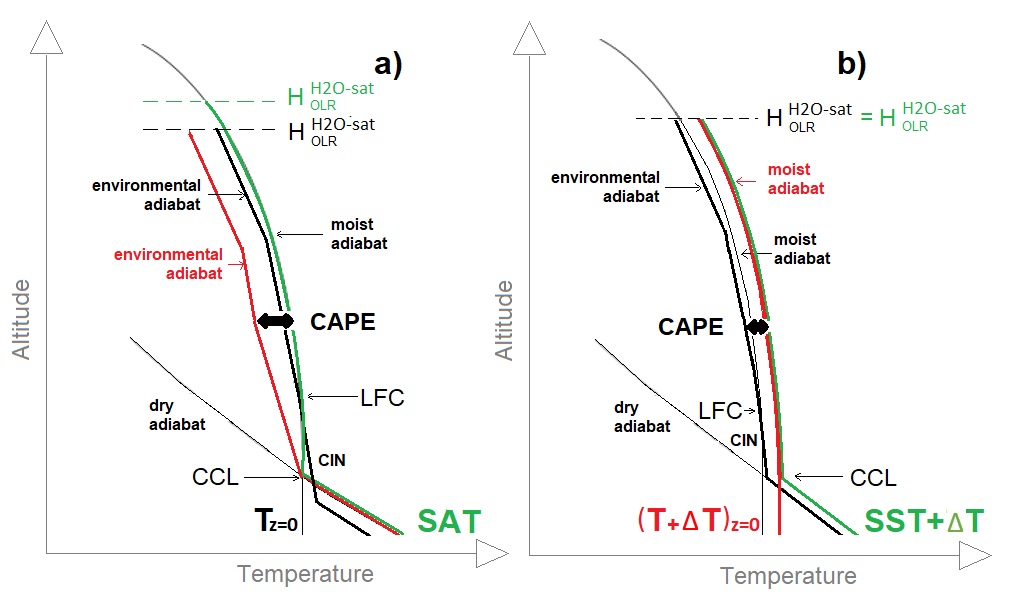
The way to make the atmosphere unstable is based on the properties of the moist adiabat as the air rises to the level of free convection. Consider as a perturbation a small increase in the temperature of the atmosphere resulting from radiative forcing induced by increasing anthropogenic emissions. The response of the atmosphere to this perturbation depends on how the derivative of the moist adiabatic lapse rate versus the temperature T_z=0 behaves.

Under the effect of increasing T_z=0, the climate system is potentially even more perturbed as the increase in CAPE is significant, compared to the unperturbed state. The minimum relative increase in CAPE as a function of T_z=0 at levels for which atmospheric pressure is 80 and 100 kPa is represented graphically. It is the ratio of the shifting of the wet adiabatic lapse rate for a 1 ° C increase in T_z=0 over the deviation between the wet and dry adiabatic lapse rates. When T_z=0 is about -40°C the moist and dry adiabatic lapse rates are confused so that CAPE is extremely sensitive to warming of the atmosphere that separates the two adiabatic lapse rates while T_z=0 increases. At low temperatures, relative increase in CAPE remains close to the minimum value because the environmental adiabat is very constrained while this constitutes a lower limit at higher temperatures, the actual value depending much on the type of climate considered. The environmental adiabat is subject to a strong seasonality in the intertropical convergence zone. In winter it approaches the dry adiabat at the horse latitudes within the dry descending branch of the Hadley cell. Therefore, instability of the atmosphere reaches its maximum, hence the moist, deep convection and the ascending branch of the Hadley cell that encircles Earth near the meteorological equator. Consequently, relative increase in CAPE that results from an increase in T_z=0 is very low, close to its minimum value.

This representation explains the strong influence of latitude on the anthropogenic forcing efficiency, which includes the Arctic amplification and the equatorial neutrality for which the positive feedback is low. Furthermore, sensitivity in CAPE to increasing Tz=0 increases with the altitude.

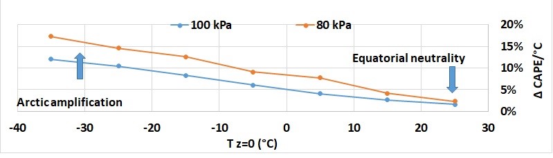
For T_z=0<-10°C, the height of convection increases nearly proportionally to the temperature perturbation. Indeed, concomitantly to the increase in the energy available to convection, a rise of H_OLR^H2O-sat increases the radiative forcing because outgoing thermal radiations are reduced. So, a positive feedback loop occurs, fixing a new H_OLR^H2O-sat. For T_z=0 ≥0°C, the height of convection is much less sensitive to the temperature perturbation. An intermediate situation occurs when -10°C≤T_z=0<0°C.

The deviation between SAT and the temperature T_z=0 of the moist adiabat at the altitude z=0 depends on the altitude of the convective condensation level. SAT at the ground or sea level may be much higher than T_z=0 , especially at low latitudes where the deviation between the dry and moist adiabats is maximum. In contrast, at high latitudes both dry and moist adiabats are close so that, SAT is close to T_z=0.

Latitudinal variations of climate response to anthropogenic forcing

As concerns the latitudinal variations of SAT resulting from the Earth’s response to anthropogenic forcing, they reach their maximum near the poles, overreaching 2.5°C. In late summer SAT goes down around -30 °C (T_z=0∿-30 °C) in the Arctic, even less in the Antarctic. An increase ΔT of the temperature perturbation induces H_OLR^H2O-sat uplift and concomitant positive feedback.

Between 30°N and 60°N and between 20°S and 40°S the SAT response to anthropogenic forcing may reach 1.5°C. In late summer SAT goes around 20 °C (T_z=0∿10 °C) and the warming results from the relative increase in CAPE that is significant so that moist convection is enhanced.

Between 30°N and 20°S the SAT response to anthropogenic forcing is generally lower than 0.5°C. In late summer SAT goes around 30°C (T_z=0∿18 °C). Relative increase in CAPE is low.

A problem is pending regarding the behavior of the Antarctic, which differs from that of the Arctic. Although the Antarctic is colder than the Arctic, the former warms less quickly than the latter, which contradicts what has been exposed previously. This suggests that, in the Antarctic, most of the time the convective condensation level is high enough to prevent any moist convective process from occurring so that properties of the moist adiabat do not apply here.

Longitudinal variations of the climate response to anthropogenic forcing

The longitudinal variation of the SAT response to anthropogenic forcing is imputable to the oceanic influence that results from atmospheric baroclinic instabilities induced from Rossby waves at high latitudes of the subtropical gyres, nearly 40°N in the North Atlantic and the North Pacific, 40°S in the South Pacific and 30°S in the South Atlantic and the South Indian Ocean. Unlike continental areas, no seasonal instability occurs here but inter-annual cycles are observed in connection with the SST anomalies. Oceanic baroclinic instabilities no longer result from a change in the environmental lapse rate. Here the thermal anomaly on the surface of the ocean enhances evaporative processes, which lowers the level of free convection (Figure b). Consequently, CAPE is much lower than that of continental areas in late summer.

SST is included between 15 and 20°C along the year, whatever the hemisphere. Supposing a thermal equilibrium at the interface ocean-atmosphere, the surface temperature T_z=0 of the moist adiabat at the altitude z=0 is around 8-12°C. Consequently, the height H_OLR^H2O-sat is only slightly modified in the perturbed state because relative variation in CAPE is low. So, the SAT response to the temperature perturbation is low, as well.

The main impacted areas are: (a) Southwest North America; (b) Texas; (c) Southeastern North America; (d) Northeastern North America; (e) Southern Greenland; (f) Europe and Central and Western Asia; (g) the region of the Río de la Plata; (h) Southwestern and Southeastern Australia, and (i) Southeast Asia.

Anthropogenic forcing in a nutshell

From idealized environmental adiabats deduced from the precipitation patterns at the planetary scale, we showed how the height H_OLR^H2O-sat responds to a small temperature perturbation of the atmosphere as a result of radiative forcing consequent to increasing anthropogenic emissions. This generates a positive feedback loop, leading to amplifying forcing effects.

Low-pressure systems may develop at the mesoscale or at the synoptic scale. During these periods of instability, the perturbation of the climate system is exerted with the concomitant warming of the surface. So the SAT response to anthropogenic forcing turns out to be the result of a succession of events with asymmetrical surface-atmosphere heat exchanges.

The response of H_OLR^H2O-sat differs according to whether atmospheric instabilities have a continental or oceanic origin. It depends strongly on the temperature of the atmosphere in the first case and the response to a small temperature perturbation is all the higher as the atmosphere is colder. In contrast, the response is almost insensitive to the temperature perturbation when instabilities have an oceanic origin. This allowed construing the latitudinal and longitudinal distribution of the SAT response to anthropogenic forcing.

Whatever the location on the planet, as a first approximation the linearity between:

1. the perturbation of the Earth’s radiation balance resulting from increasing anthropogenic emissions
2. the vertical displacement of H_OLR^H2O-sat under the effect of the resulting positive feedback loop
3. the variation of SAT

allows predicting the evolution of the climate system according to the future anthropogenic forcing from the sensitivity of the Earth’s response to the anthropogenic forcing observed since 1970.

However, this is only applicable in the limited context of a climate system that remains little modified. This is not the case where polar ice caps melt. The positive feedback loop reacts synergistically with the reduction of albedo due to melting of the pack ice in summer.

From the stable oxygen isotopic compositions of speleothems, the evolution of long-term rainfall oscillation during the Holocene can be reconstructed. This study highlights the quasi-resonance of the equatorward migration of the summer Inter Tropical Convergence Zone (ITCZ) during the Holocene, because of the progressive decrease of the thermal gradient between the low and high latitudes of the gyres. The latitudinal shift of the summer ITCZ and the shrinkage of the Hadley cell in response to changes in the thermal gradient is of the utmost importance in predicting the expansion of deserts resulting from the melting of sea ice due to anthropogenic warming.

Glossary

The Intertropical Convergence Zone, or ITCZ, is the region that circles the Earth, near the equator, where the trade winds of the Northern and Southern Hemispheres come together. The Hadley cell is a global-scale tropical atmospheric circulation that features air rising near the Equator, flowing poleward at a height of 10 to 15 kilometers above the earth’s surface, descending in the subtropics, and then returning equatorward near the surface.

Jet-streams are fast winds aloft blowing from west to east. Along a curved and sinuous path, they play a major role in atmospheric circulation as they participate in the formation of depressions and anticyclones at middle latitudes, which then move under these powerful atmospheric currents.

Positive feedback loops amplify changes in a dynamic system; this tends to move the system away from its equilibrium state and make it more unstable. Negative feedbacks tend to dampen changes; this tends to hold the system to some equilibrium state making it more stable.

The adiabatic lapse rate is, in the Earth’s atmosphere, the variation of air temperature with altitude (in other words, the gradient of the air temperature). Adiabatic means that a mass of air does not exchange heat with its environment (other air masses, relief). If we exclude condensation (formation of clouds and precipitation) and vaporization, the lapse rate of the atmosphere depends only on the pressure.

The moist adiabatic lapse rate is the rate at which the temperature of a parcel of saturated air decreases as the parcel is lifted in the atmosphere. The moist adiabatic lapse rate is not a constant like the dry adiabatic lapse rate but is dependent on parcel temperature and pressure.

Thermal fluxes that impact the surface temperature of the perturbed climate system are asymmetrical depending on whether they are incoming or outgoing fluxes. Incoming fluxes warm the surface of the Earth quasi-instantaneously since the thermal energy accumulated while the climate system is perturbed as a result of radiative forcing is partially trapped up to H_OLR^H2O-sat. A transient thermal equilibrium between the surface and the atmosphere occurs rapidly because of precipitations and sensitive heat fluxes resulting from the low-pressure systems. On the other hand, when the atmosphere becomes stable again, the thermal exchanges that make the surface temperature tend to decrease to recover the value it should have kept if the climate system had not been perturbed are much slower. The surface-atmosphere system behaves like a quasi-isolated thermodynamic system because exchanges are mainly ruled by evaporative processes. This implies that the heat accumulated is conserved on a synoptic scale.

As highlighted by the Nimbus Michelson interferometer experiment, emission of outgoing longwave radiation in the saturated absorption bands of water vapor occurs from a surface whose temperature is nearly 260 K, that is, close to 4.3 km high. Indeed, longwave radiation emitted from the surface of the Earth in the saturated absorption bands of water vapor is such that the optical path is much lower that the thickness of the free convection layer. So, thermal radiation scatters up to the level of emission of outgoing longwave radiation in the saturated absorption bands of water vapor (H_OLR^H2O-sat) before escaping to the cosmos. The emission spectrum is that of a truncated black body radiation so that composition of the atmosphere at H_OLR^H2O-sat does not matter whether it is the density of clouds, their type or composition.

The SAT response to anthropogenic forcing reflects the variations of H_OLR^H2O-sat. Uprising of H_OLR^H2O-sat increases radiative forcing resulting from water vapor and clouds because outgoing thermal radiations are cooled. Lowering of the temperature of the emission surface increases the temperature of the atmosphere under H_OLR^H2O-sat. At mid-latitudes a 46 m uprising of H_OLR^H2O-sat generates an increase in SAT of 0.1 °C.