The climate during Holocene, which began with the interglacial period about 12500 years ago, can be studied from proxies of solar irradiance and Earth’s average temperature in both hemispheres. Superimposed on oscillations are several distinct climate steps which appear to be of widespread significance, the most prominent being observed 8.2 Kyr, 5.5-5.3 Kyr and 2.5 Kyr (Kyr=103 years) BP. These events, which are recognized as part of the millennial scale quasi-periodic climate changes, alongside the Dansgaard–Oeschger (D-O) cycles, and are characteristic of the Holocene [O’Brien et al, 1996; Bond et al, 1997; Bianchi and McCave, 1999; de Menocal et al, 2000; Giraudeau et al, 2000].
As observed during the glacial-interglacial era, the temperature of the earth’s surface is subject to the resonance of gyral Rossby waves that results from solar and orbital forcing. From this follows the resonant nature of the climate system. The forcing is all the more efficient as its period is closer to one of the resonance periods, the latter being locked in subharmonic mode (Pinault 2018d, 2020a, 2021a).
During the Holocene that began 12,000 years ago with the end of the last glaciation, climatic variations, which can be observed from the analysis of ice cores, speleothems, pollen, and tree-ring data, occur mainly in two frequency bands.
Contents
The band 576-1152 years
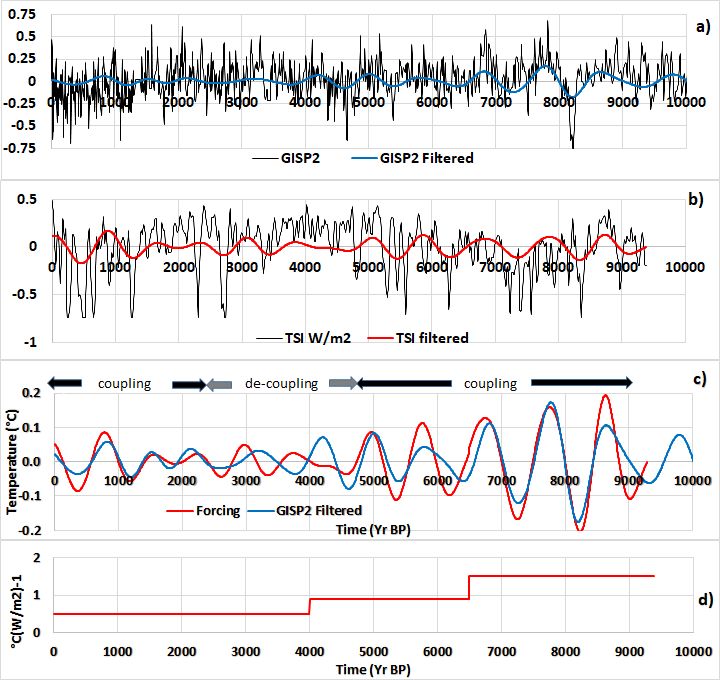
In the North Atlantic, there are similarities between the Total Solar Irradiance (TSI) multiplied by the forcing efficiency and the global temperature into the band 576-1152 years characteristic of the 64×12=64x3x22=768 year period whose subharmonic mode is 3×22 (number of turns made during half a period). The two curves show a similarity mainly over the interval covering 9000 to 6000 years BP, that is, when the forcing efficiency is maximum.
The forcing efficiency, that is, the sensitivity of the global temperature (°C) to the solar insolation (W/m2), varies over time: equal to 1.5 °C(W/m2)-1 between 9000 and 6500 years BP, it decreases to 0.5 °C(W/m2)-1 after 5000 years BP. This is because the response of the gyre to the variations in the TSI is all the more enhanced as the gradient of the sea water temperature between low and high latitudes of the gyre is steeper. At the beginning of the Holocene, the pack ice extended further south, which explains the high radiative forcing efficiency. Then, gradual withdrawal of the pack ice made the positive feedback of the polar current on the thermocline depth less efficient.
Between 5000 and 2500 years BP the amplitude of solar irradiance into the band 576-1152 years decreases, and the Gyral Rossby Wave (GRW) disassociates from the solar irradiance cycle, both the amplitude and period. During this period of decoupling the GRW does not weaken because of the remanence of geostrophic forces throughout the gyre and along the drift currents (collective effects of the gyres in the various frequency bands), but its period lengthens, which indicates that the centroid of the gyre drifts poleward. The GRW is coupled to the solar cycle again between 2500 years BP and present during the upsurge of the solar cycle. Therefore the resonance of the 3×22 subharmonic mode GRW appears to be the main driver of climate variability during the Holocene.
The band 96-192 years
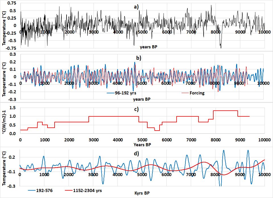
GRWs are resonantly forced within the 96-192 year band, which results from the Gleissberg cycle of the Sun. The forcing efficiency varies a lot during the Holocene, mainly during the periods of low solar activity during which it weakens drastically.
Evolution of Glaciers in the Northern Europe and the Climatic Transitions during the Holocene
As the extension of glaciers in Norway reacts quickly to the forcing of the climate system, their evolution offers opportunities to study climate variability during the Holocene (Pinault, 2021b). The evolution of glaciers reflects the subharmonic modes of the North Atlantic gyre, so that the mechanisms involved in teleconnections can be revealed, essentially the change in the atmospheric circulation over the North Atlantic from the mid-Holocene, then the successive abrupt cooling events that have occurred during the Holocene, including Bond events such as the Late Antique Little Ice Age (LALIA) and the Little Ice Age (LIA). In this case, it is the highlighting of an anharmonic mode that will make it possible to deepen the mechanisms which are responsible for them.
Abrupt cooling events
Pollen data from 11 lakes, plus July pollen/tree-ring data for the past 7500 years obtained in Northern Fennoscandia (Helama et al., 2012) clearly highlight subharmonic modes of the surface temperature in Northern Europe.

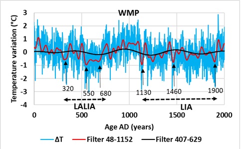
In addition to the 5 subharmonic modes corresponding to the subharmonic numbers n2 to n6, an anharmonic mode is highlighted at 444 years. This broad peak highlights successive cooling periods (signal filtered in the 407–629-year band), namely, the Little Ice Age (LIA) that mainly occurred in 1130, 1460 and in 1900 AD and the Last Antique Little Ice Age (LALIA) that occurred in 320 and in 550–680 AD, separated by the Medieval Warm Period (MWP).
Abrupt cooling events are favored when the western boundary current is slowing down. Presumably, the current of the gyre in its northernmost part before branching off to the north increases its density so that it plunges under surface water, not very salty because of the progressive melting of the pack ice promoted by the northward advection of warm air. It follows a significant cooling of northern Europe. The current of the gyre resurfaces as soon as it warms up and thermal exchanges are restored between the ocean and the continents. These transitions are rapid because the density of the surface layer and the underlying current of the gyre remain close, which favors the overturning.
The Speleothems, Witnesses of the Evolution of Precipitation
Now, we are trying to quantify the amplitude of variations in precipitation during the Holocene in different regions of the globe to highlight the evolution of large-sale atmospheric circulation. This study is based on the use of speleothems available in the database developed within the framework of the Speleothem Isotopes Synthesis and AnaLysis (SISAL) project. The method consists in taking advantage of the stable oxygen isotopic composition (18O) in the calcite/aragonite of cave concretions, which involves processes that control equilibrium and kinetic fractionation of oxygen isotopes in water and carbonate species.
Because of the observed correlation between the decrease in rainfall 18O values and the increase in the amount of rain (Dansgaard, 1964), the so-called “amount effect” (Rozanski et al., 1993, Bony et al., 2008, Risi et al., 2008), precipitation amount can be deduced from 18O measurements in speleothems.
Variations in 18O Concentration in Speleothems According to the Latitude (Pinault and Pereira, 2021 c)
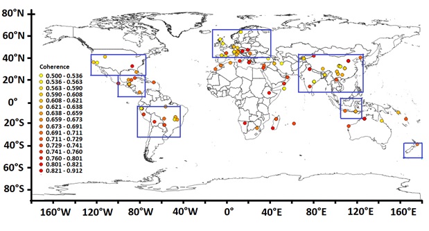
The location of the summer Inter-Tropical Convergence Zone (ITCZ) is deduced from the amplitude of rainfall oscillation (18O per mil) versus the latitudes. In North America, the summer ITCZ was positioned 37° N 10,000 years BP (c) to shift to 21° N 2000 years BP (a), i.e., the same location as in mid-Holocene, albeit less accurate (b). In South America, the summer ITCZ was 25° S 10,000 years BP (f) with a shift to 4° S 2000 years BP (d). Here again, the intermediate value lacks precision due to the scarcity of speleothems. As for Asia, the summer ITCZ was placed 42° N 10,000 years BP (i) with a shift to 25° N 2000 years BP (g). However, equatorward migration of the summer ITCZ has been slower than in the previous two cases as it was still ongoing in the mid-Holocene when the summer ITCZ was located 34° N.
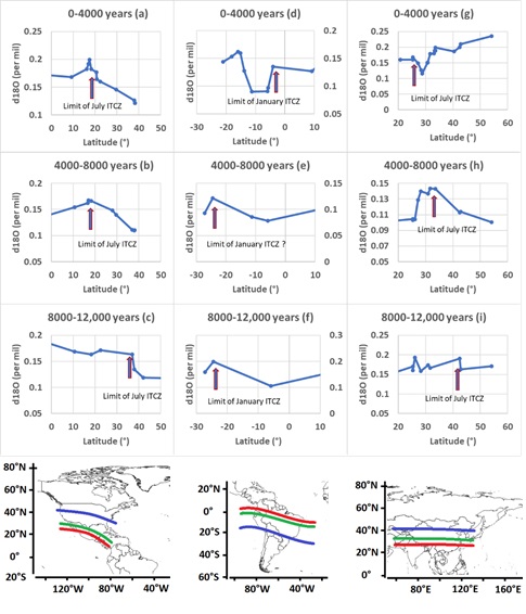
The oscillation amplitude is high in Asia over the region located between 43° N and 10° N, regardless of the subharmonic mode. This region is dominated by widespread and persistent subtropical high-pressure cells with the associated circulation patterns that propitiate the formation of low- to mid-latitude arid zones in Asia. This probably makes that region very sensitive to changes in monsoon circulation.
The tropical Southeast Asia region is not subject to rainfall oscillation. However, the increased amplitude in the early Holocene observed for the subharmonic mode n5 suggests an encroachment of the January ITCZ over that region located between 5° N and 15° S (f).
Despite being also located inside the Hadley cell, the Central American region experiences strong rainfall oscillation for all subharmonic modes because of the quasi-permanent encroachment of the ITCZ in July. It is therefore the latitudinal oscillation of the July ITCZ which seems to occur for all subharmonic modes, tuned according to the different periods.
Thus, the ITCZ migrated equatorward until it reached an equilibrium position fixed by the current thermal gradient. This clearly highlights the vulnerability of the regions exposed to the narrowing of the Hadley cell because of the melting of the ice caps that is reducing the thermal gradient between the low and high latitudes of the gyres. In arid regions bordering deserts, the shifting of moisture flow out of these regions has important implications for probable changes induced by global warming (Pinault, 2021c).
Variations in 18O Concentration in Speleothems in the Tropical Pacific
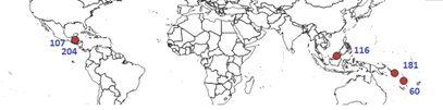
Sixteen high resolution speleothems are available at five sites. Sites 181 and 60 are in the tropical South Pacific convergence zone. 18O in Borneo rainfall (site 116) is a robust proxy of regional convective intensity and precipitation amount, both of which are directly influenced by ENSO activity. These three sites, being located to the west of the tropical basin, are negatively correlated with the ENSO: precipitation decreases during ENSO. East of the tropical basin, the sites 107 and 204, located in the convection zone, are positively correlated with ENSO.
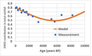
The contribution of ENSO to precipitation from the speleothems is obtained as follows. The signals are first filtered in the 2-7 years band representative of ENSO, then in the band 0.5-7 years which integrates all precipitation. Then, for each period considered, the contribution of ENSO to precipitation is obtained by dividing the standard deviation of the filtered signal into the band 2-7 years by the standard deviation of the filtered signal into the band 0.5-7 years.
ENSO activity decreases in the middle of the Holocene, a result widely accepted by the scientific community nowadays. However, the precision of the measurement results allows a straightforward interpretation from the decomposition into subharmonic modes of 18O concentration in the GRIP ice core record used as a paleo proxy of the amplitude of GRWs.
Evolution of ENSO activity during the Holocene strengthens the interpretation given from 18O concentrations in short-lived individual foraminifera in a sediment core sampled from the eastern equatorial Pacific near the Galapagos Islands (Pinault, 2021a).
References
Helama, S.; Seppä, H.; Bjune, A.E.; Birks, H.J.B. Fusing pollen-stratigraphic and dendroclimatic proxy data to reconstruct summer temperature variability during the past 7.5 ka in subarctic Fennoscandia. J. Paleolimnol. 2012, 48, 275–286.
Matskovsky, V.V.; Helama, S. Testing long-term summer temperature reconstruction based on maximum density chronologies obtained by reanalysis of tree-ring data sets from northernmost Sweden and Finland. Clim. Past 2014, 10, 1473–1487.
Dansgaard,W. Stable isotopes in precipitation. Tellus 1964, 16, 438–468.
Rozanski, K.; Araguás-Araguás, L.; Gonfiantini, R. Isotopic patterns in modern global precipitation. In Climate Change in Continental Isotopic Records; Swart, P.K., Lohmann, K.L., McKenzie, J., Savin, S., Eds.; American Geophysical Union: Washington, DC, USA, 1993; pp. 1–37.
Bony, S.; Risi, C.; Vimeux, F. Influence of convective processes on the isotopic composition (18O and D) of precipitation and water vapor in the tropics: 1. Radiative-convective equilibrium and Tropical Ocean–Global Atmosphere–Coupled Ocean-Atmosphere Response Experiment (TOGA-COARE) simulations. J. Geophys. Res. Space Phys. 2008, 113, 19305.
Risi, C.; Bony, S.; Vimeux, F. Influence of convective processes on the isotopic composition (18O and D) of precipitation and water vapor in the tropics: 2. Physical interpretation of the amount effect. J. Geophys. Res. Space Phys. 2008, 113, 19306
Glossary
Positive feedback loops amplify changes in a dynamic system; this tends to move the system away from its equilibrium state and make it more unstable. Negative feedbacks tend to dampen changes; this tends to hold the system to some equilibrium state making it more stable.