Contents
Solar cycles
Changes in solar irradiance are reflected by the number of sunspots that recent satellite measurements confirm. The spot number, which is accurately known since the 17th century, shows that solar irradiance varies mainly in four bands. They are the Schwabe cycle of 9-13 years, the Jupiter – Saturn cycle of 59 years, the Gleissberg cycle of 90-110 years and the DeVries and Suess cycle of 180-220 years. Cosmogenic isotopes confirm the existence of these and other longer solar cycles such as the Hallstattzeit cycle of 2,300 years.
The 59-year cycle results from the shifting of the center of gravity of the solar system relative to the center of the sun, in relation to periods of rotation of the largest planets, i.e. Jupiter and Saturn. The Gleissberg cycle, which was discovered in 1958, possibly is a modulation of the amplitude of the 11-year Schwabe cycle, which itself results from the differential rotation of the convection zone of the sun, periodically inducing a deformation followed by the consolidation of the magnetic flux tubes. The origin of the cycles of longer periods is not known with certainty.
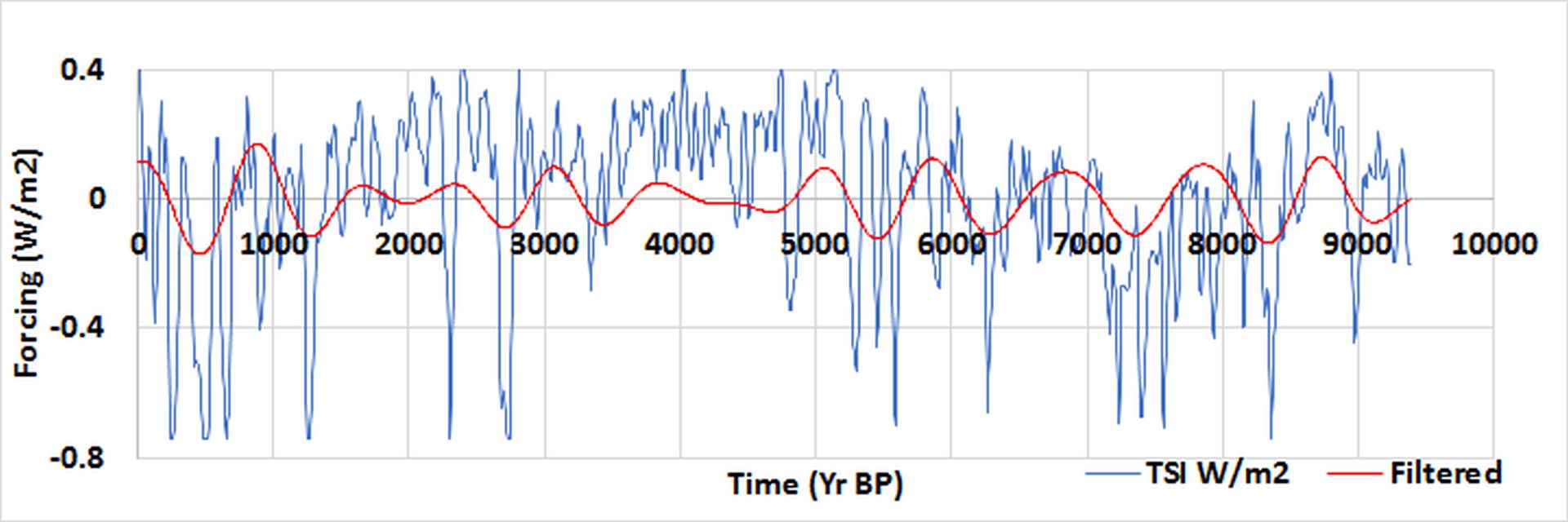
Understanding the temporal variation of cosmic radiation and solar activity during the Holocene allows specifying the solar-terrestrial relationship. 10Be and 14C which are stored in polar ice cores and tree rings, offer the opportunity to reconstruct the history of cosmic radiation and solar activity. In series obtained by Steinhilber et al., [2012] different 10Be ice core records from Greenland and Antarctica are combined with the global 14C tree ring record to provide total solar irradiance variations (W/m2).
The last few million years have been punctuated by many abrupt climate transitions. Many of them occur on time-scales of centuries or even decades. The ability of climate to change abruptly has been one of the most surprising outcomes of the study of Earth history [e.g., Jouzel et al 1987, Taylor et al 1993; Petit et al 1999, Dansgaard et al 1993; Alley, 2000, Jouzel et al 2007].
Climate changes at the planetary scale are responses to external forcing mechanisms, that’s what we strive to show in this chapter. The role of the Sun in climate variability, and specifically solar irradiance fluctuations which reflect the internal dynamics of the Sun but also orbital forcing that alter the net radiation budget of the Earth are frequently referred [e.g. Magny, 1993, Karlén and Kuylenstierna, 1996, Chambers et al., 1999, Bond et al., 2001, Gavin et al., 2011]. Nevertheless, the internal mechanisms involved in long-term climate variability are poorly understood. The idea often mentioned that the deep ocean is the only candidate for driving and sustaining long-term climate change (of hundreds to thousands years) because of its volume, heat capacity, and inertia [e.g. Maslin et al, 2001], can easily be counteracted in the glow of the present results. Indeed, variations in the flow and temperature of deep water that is known to have a direct effect on global climate is a consequence of a mechanism of much greater scope involving the resonance of sub-tropical oceanic gyres.
Milankovitch cycles
Milutin Milankovitch, of Serbian origin, was at once an astronomer, geophysicist and climatologist. In 1911, Milankovitch was interested in glacial periods of the Pleistocene, a geological epoch from 1.8 million years to 11,500 years before our era. It is characterized by prolonged glaciations, glaciers covering the continents, interrupted by short interglacial periods with temperate climate. Milankovitch established a mathematical theory of climate. In his calculations, he included information on small variations in the inclination of the axis of the Earth, and small orbital changes caused by the gravity of other planets, Jupiter and Saturn essentially, each of these orbital variations with a definite period. Milankovitch proposed that changes in the intensity of the solar radiation received by the Earth are due to three basic factors: the eccentricity with a period of 413,000 and 100,000 years, the inclination with a period of 41,000 years, the precession with periods of 23,000 and 19,000 years. The tables he drew are still true, confirmed by more recent calculations.
Since 1976, inspection of deep ocean cores has confirmed the Milankovitch theory. We can reconstruct changes in ice volume using measurements of oxygen isotope in the calcite shells of foraminifera. Indeed, variations in 18O in seawater can be correlated to changes in volume of ice. During the glacial period, the sea level was 130 m below the current level. Accordingly 18O of the ocean was 1.5 per thousand higher than what it is today. Measuring 18O in the shells of foraminifera allows to reconstruct changes in the volume of ice on the scale of million years. Thus, the climate could be restored over a period of 5.3 million years, by means of a graphical correlation algorithm that takes into account the constraints on sedimentation rates, more than 50 cores coming from abysses in the three oceans.
Orbital forcing
A perspective on climate variability and orbital forcing, i.e. the precession, the obliquity and the eccentricity, what are commonly named Milankovitch parameters, arises huge problems and there is currently no consensus on the responsible mechanism. On one hand the impact of orbital variations on climate seems not proportional to the amplitude of solar irradiance variations. On the other hand, over the past 800,000 years, the period of oscillation of glacial-interglacial that dominated is 100,000 years, showing it is mainly subject to eccentricity parameter. During the interval from 3.0 to 0.8 million years before our era, the period of 41,000 years prevailed, corresponding to changes in the obliquity of the Earth, what is named the transition problem.

The observations suggest that a resonance phenomenon occurs, filtering out some frequencies in favor of others. This hypothesis, issued for several decades, has so far not found plausible physical explanation. This suggests a priori that the gyral resonance is the missing link to solve this riddle. Effectively, there exists a link between orbital forcing and the amplitude of the long baroclinic waves around the gyres.
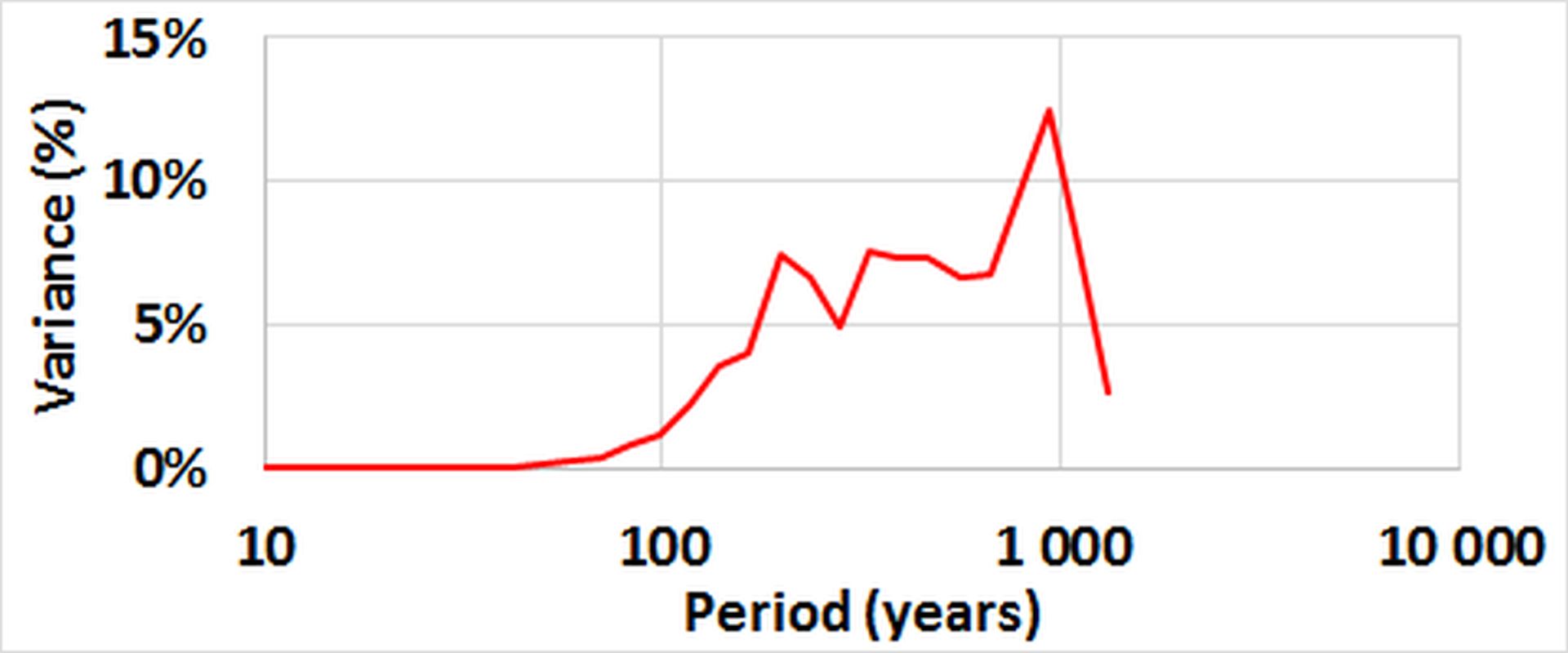
Owing to the sub-harmonic mode locking of coupled oscillators with inertia, periods of gyral Rossby waves forced by the Milankovitch cycles are a multiple of shorter periods that meet the cycles of solar radiation (Pinault, 2018c). Thus, the sub-harmonics form a sequence whose average periods are multiples of 768 years, the dominant period of the gyral resonance during the Holocene. But, contrarily to what occurs during the Holocene, the narrow frequency bands of orbital forcing complicate the interpretation of the coupling because of the deviation between the frequencies of forcing and the natural frequencies of gyral Rossby waves.
To tune the natural frequency of gyral Rossby waves to the forcing frequency while keeping the wavenumber, the latitude of the centroid has to be shifted. Because several components tuned to their own orbital frequency coexist, instabilities occur around the gyre but the resonance conditions are no longer fulfilled accurately. In this way, the efficiency of forcing depends on the latitude of the centroid of the gyral Rossby waves, which oscillate on either side of their mean value.
Ice and sediment core records allow a detailed study of the glacial-interglacial era in the various characteristic bands.
The origins of glacial-interglacial oscillation from the Milankovitch cycles can be understood from these two extreme cases:
1) for the occurrence of an interglacial period, an extreme orbital configuration results from high eccentricity (the Earth’s orbit is an ellipse), large inclination and low Earth – Sun distance in summer. It follows very contrasting seasons, thus warming as the main variable is the amount of radiation received in summer at high latitudes of the northern hemisphere.
2) on the contrary, for the glacial period the orbit of the Earth is nearly circular (low eccentricity) with a low inclination and a large Earth – Sun distance in summer. This results in a low seasonal contrast and a favorable cooling configuration.
On longer time scales, sediment cores show that the cycles of glacial and interglacial periods are episodes of a long ice age that began with the glaciation of Antarctica about 40 million years ago. However, these glacial and interglacial cycles primarily began about 3 million years ago with the growth of continental ice caps in the Northern Hemisphere. During the period from 3.0 to 0.8 million years before our era, the period of 41,000 years prevailed, corresponding to changes in the inclination of the Earth. Over the past 800,000 years, the period of oscillation of glacial-interglacial that dominates is 100,000 years, corresponding to the evolution of the eccentricity of the Earth, which is however of lower amplitude that is the obliquity.
Radiative forcing efficiency
One of the most surprising property of radiative forcing, in W/m2, is the variability of its efficiency , that is to say its impact on the Earth’s global temperature, in °C, depending on the periods. The application of the Stefan-Boltzmann law tells us that, if we consider that our planet behaves as a black body, that is to say, its emission spectrum in the infrared only depends on its temperature, the efficiency of solar forcing is 0.22 °C/(W/m2). Yet this efficiency can be increased considerably since climate archives teach us that it is up to 5 °C/(W/m2) in the band 73.7-147.5 Kyrs during the glacial-interglacial periods, a consequence of orbital forcing. On the other hand, equal to 1.5 °C/(W/m2) in the band 576-1152 years at the beginning of the Holocene because of solar forcing, it is 0.5 °C/(W/m2) nowadays.
Such a change in radiative forcing efficiency assumes a positive feedback loop in the climate system because the variability of the incident short wavelength radiation is far too low to impact overall temperature. To explain the resonant character of the climate system it is necessary to involve the oceans through the modulated response of subtropical gyres (Pinault, 2018d). The amplifying effect of solar and orbital forcing comes from the positive feedback exerted by the polar current of the gyral Rossby wave: the oscillation of the thermocline is amplified by the polar current which warms or cools, as the western boundary current accelerates or slows down. The amplification is tightly controlled because limited by the sea water’s ability to warm at low latitudes and by the resulting cooling of upwelling along the eastern boundary current of the gyre.
Thus, the amplifying effect of solar and orbital forcing shows that the transfer of heat from the equator to the poles occurs with varying efficiency. Acceleration or, conversely, slow-down of the polar current of the gyral Rossby wave impacts sea surface temperature anomalies, especially at high latitudes of the subtropical gyres. These thermal anomalies act either as a heat source, or, contrarily, as a heat sink. The resulting perturbation behaves like an isolated thermodynamic system: heat transfer between oceans and continents occur until equilibrium is established between the oceanic and continental anomalies.
The amplification phenomenon is all the more significant as the sea surface temperature at high latitudes is lower, which has the property to increase feedback. Thus the forcing efficiency depends on the forward motion of sea ice in both hemispheres, which explains its evolution during the Holocene. Regarding the orbital forcing whose bandwidth is narrow, its efficiency is highly dependent on the difference between the period of forcing and the natural period of the gyral Rossby wave. Thus in the period extending from 3.0 to 0.8 million years before our era, the period of 41,000 years predominates, corresponding to changes in the tilt of the earth. Over the past 800,000 years, the dominating period of oscillation of glacial – interglacial is 100,000 years, corresponding to changes in the eccentricity of the earth.
Glossary
Cosmogenic isotopes are produced by cosmic rays in the upper atmosphere, forming rare isotopes of hydrogen (3H) and produces helium (3He), beryllium (10Be), carbon (14C), neon (21Ne), aluminum (26Al), and chlorine (36Cl). Isotopic abundance reflects solar activity: during periods of high activity cosmic rays are deflected out the solar system and therefore produce less cosmogenic isotopes.
[i] Relationship between benthic foraminifera δ18O and volume of polar ice
Ice of the polar caps is depleted in H2 18O about 30-40 ‰ (δ18O ~ – 40 ‰ = – 4%) compared to ocean water. Indeed, the water vapor transported from low latitudes toward the poles undergoes isotopic fractionation (depletion of 18O, heavy oxygen isotope consisting essentially of 16O) during successive condensations, all the more important as temperature decreases. As the total amount of H2 18O (oceans + caps) is constant, the more bulky the caps (at constant δ18O), the more concentrated in H2 18O seawater is, by difference. The volume of the caps and the δ18O in seawater therefore vary in the same direction and proportionally.
Relationship between δ18O in the oceans and δ18O of benthic foraminifera
Benthic foraminifera are protozoa that live on the ocean floor and synthesize a carbonate shell with isotopic composition that depends on the water temperature and δ18O of water. As the water temperature varies only slightly at depths, variations in δ18O in the shells depend only of those of water.
Upwelling. Here, this term indicates an upward flow of deep water, therefore cold. The upwelling is associated with the functioning of tropical resonant waves.
Baroclinic wave. In contrast with barotropic waves that move parallel to isotherms, baroclinic Rossby or Kelvin waves cause a vertical displacement of the thermocline, often of the order of several tens of meters. The seconds are usually slower than the first.