Contents
- Isotopic signature of the carbon dioxyde of combustion gases
- Anthropogenic CO2 concentration in the atmosphere.
- Interpretation of results
Isotopic signature of the carbon dioxide of combustion gases
Carbon has three isotopes: carbon-12, 13, and 14. The Carbon-12 is by far the most abundant, carbon-13 is about 1%, and carbon-14, only 1 in 1 billion atoms of carbon into the atmosphere.
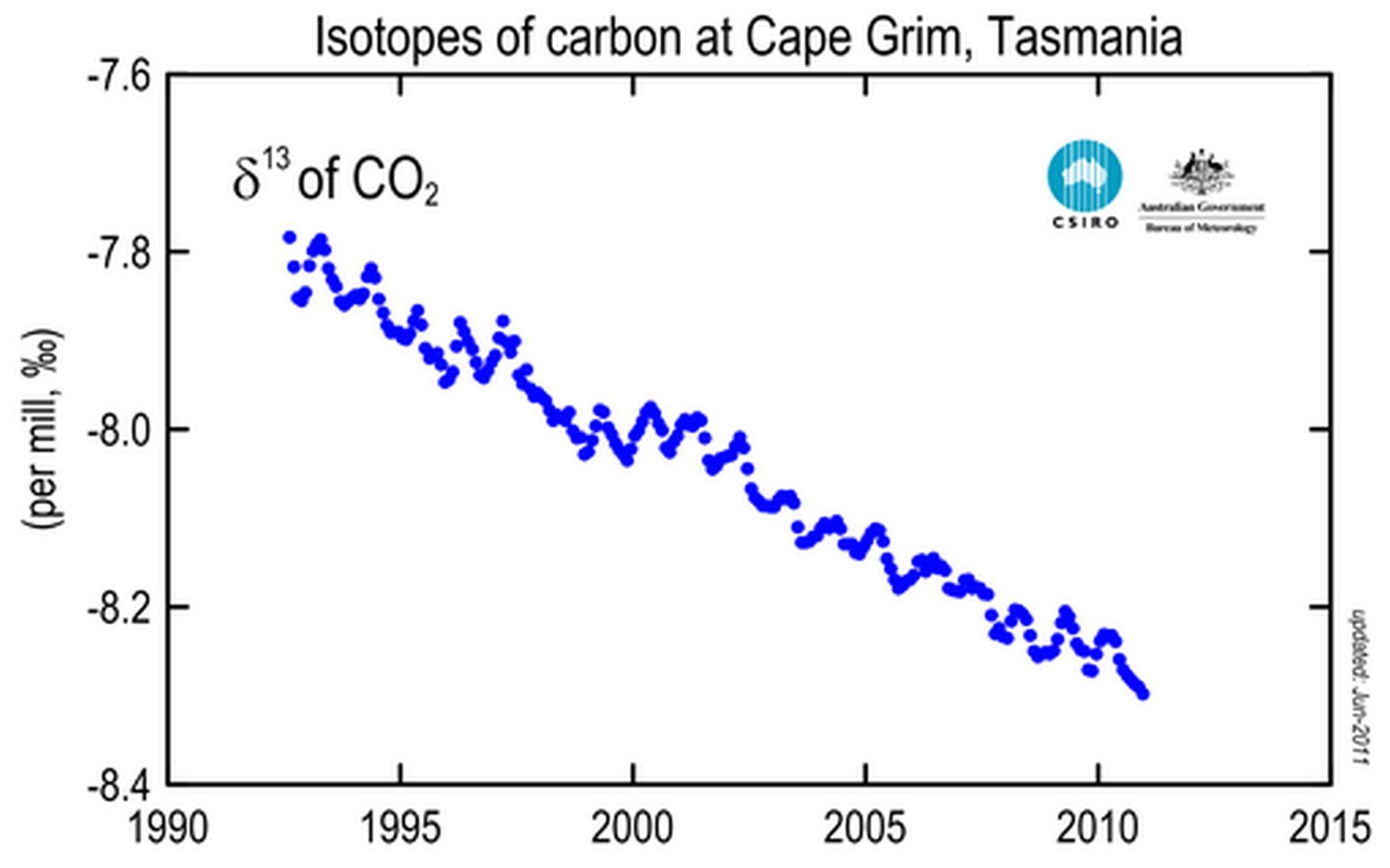
The CO2 produced by burning fossil fuels or wood has a different isotopic composition from CO2 in the atmosphere, because plants have a preference for the lighter isotopes, which lowers the carbon isotope ratio-13 / carbon-12. Given that fossil fuels come from plants, they all have roughly the same isotope ratio – about 2% lower than in the atmosphere. As CO2 from combustion gases mixes with atmospheric CO2, it lowers the isotope ratio.
Anthropogenic CO2 concentration in the atmosphere.
.

The proportion of biogenic CO2 (as opposed to CO2 from the oceans and volcanoes) is derived from the isotope ratio of carbon-13, knowing the global consumption of fossil fuels, coal, oil and gas (http://www.tsp-data-portal.org/Energy-Production-Statistics#tspQvChart ).
Considering the isotope ratios of carbon (αc = -25 ‰), heating oil (-26.5 ‰ = αo), natural gas (αg = -45 ‰) and the amount of CO2 (ppmv = parts per million by volume for 100,000 TWh) emitted by coal (ηc = 4.24), heating oil (ηo = 3.35) and gas (ηg = 2.54), depletion of 13CO2 into the atmosphere due to combustion gases , is:
13CO2combustion = ∑i=1,N[Cci× αc× ηc+ Coi× αo× ηo+ Cgi× αg× ηg] (1)
where Cci , Coi , Cgi represent the consumption during the year i of coal, heating oil and gas. N is the lifetime in the atmosphere (in years) of 13CO2.
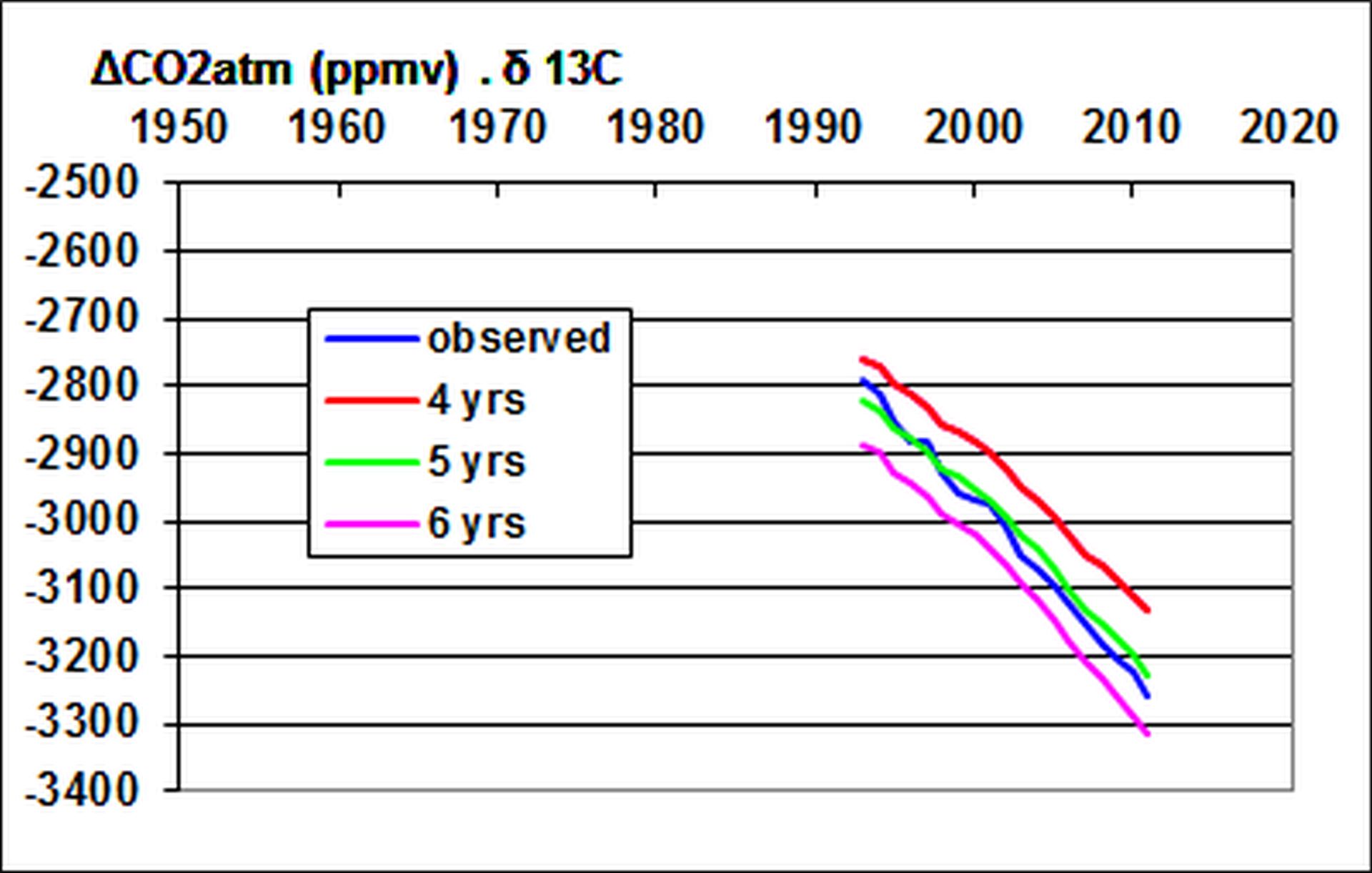
To express the 13CO2 depletion in the atmosphere, it must be added to 13CO2combustion the contribution of 13CO2natural from the oceans and volcanoes:
13CO2natural = [CO2total-∑i=1,N[Cci× ηc+ Coi× ηo+ Cgi× ηg]]× αn (2)
where αn is the carbon isotope ratio in the atmosphere before the industrial revolution, in the range of -6.5 to -7 ‰. Comparing 13CO2natural with the measured 13CO2, product of the CO2 concentration in the atmosphere by the isotope ratio of carbon-13, it follows the lifetime N of 13CO2: N = 5 to 8 years depending on the isotope ratio considered before the industrial era.
This lifetime of 13CO2 originating from combustion gases is the duration of exchanges between the atmosphere and the various reservoirs (oceans, biosphere) until the standardization of the isotopic signature of carbon dioxide due to interchangeability of 13CO2 and 12CO2 molecules.
For the lifetime of CO2 from combustion gases in the atmosphere, the calculation of its impulse response is required, that is to say, the response of the atmosphere to a carbon dioxide pulse until the complete vanishing of the effects of the pulse. The simplest form of this impulse response is the rectangle function Rec (t) such that:
Rec(t)=1 if 0≤t≤N’, Rec(t)=0 if t<0 or t>N’ (3)
where N’ is the duration (in years) of the impulse response. Consider a rectangular impulse response is to assume that the carbon dioxide concentration from the pulse is maintained throughout this period until its complete vanishing.
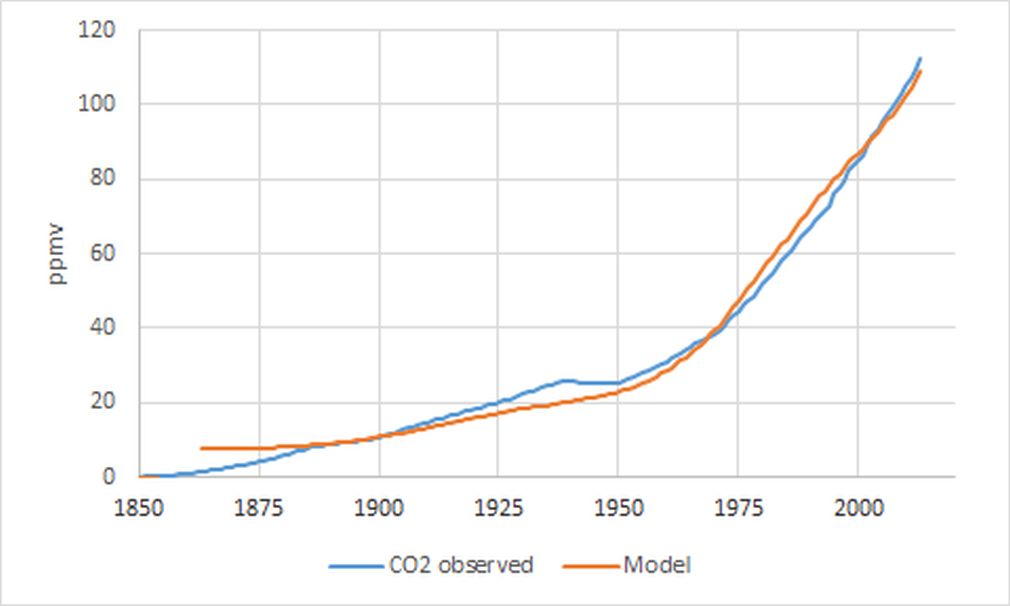
Carbon dioxide is originating from 2 sources, combustion gases on the one hand and the degassing of the oceans due to warming of gyral Rossby waves at mid-latitudes on the other hand, calculation of N’ amounts to solve the linear system:
∆CO2obs = IT*∆T+∑i=1,N’[Cci× ηc+ Coi× ηo+ Cgi× ηg] (4)
where the symbol * represents the convolution product. At time t, IT*∆T = ∑i=1,N’’IT(i).∆T(t-i) where N’’ is the duration of the impulse response of the atmosphere to a temperature pulse (an increase in temperature during one year). ∆T is the change in global temperature considered here as representative of the sea surface temperature anomalies at mid-latitudes.
Solving (4) consists in calculating the positive impulse response IT(t):
IT(t) ≥ 0 if 0 ≤ t ≤ N’’, IT(t) = 0 if t<0 or t>N’’ (5)
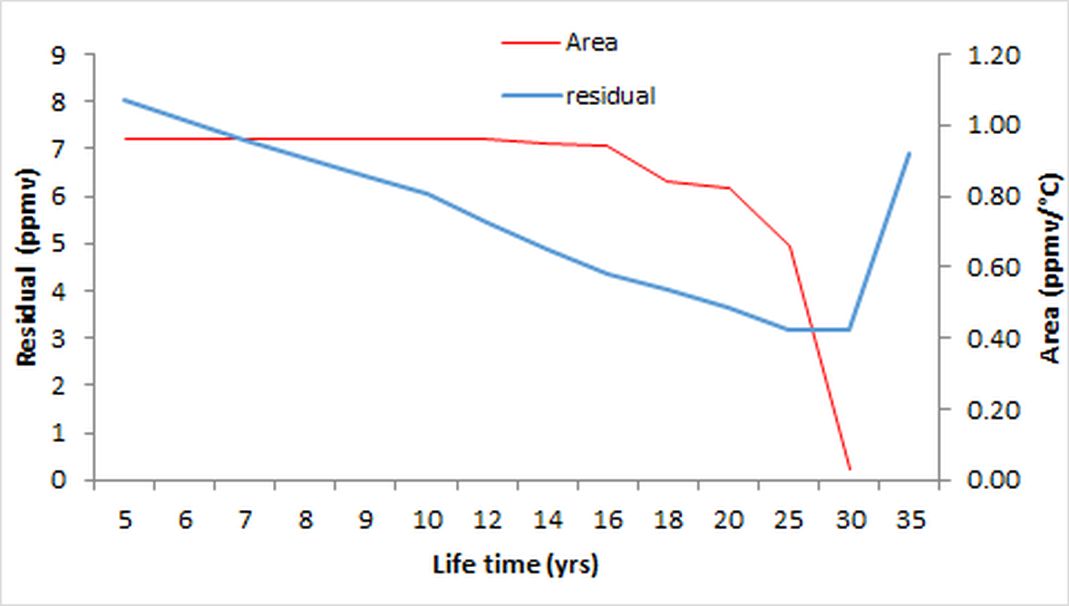
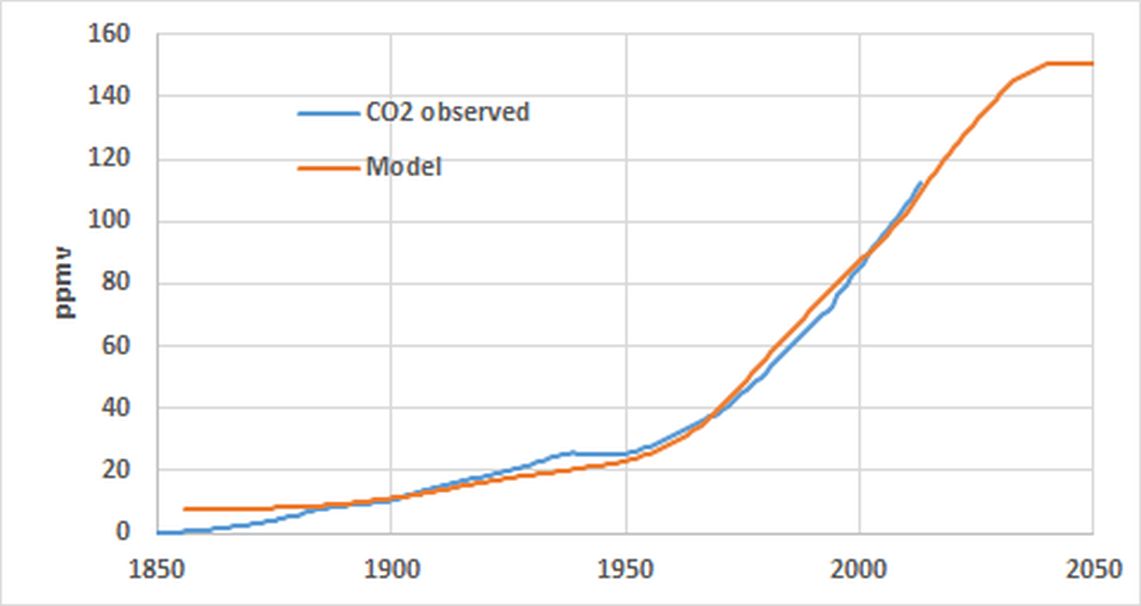
and the lifetime N’ of anthropogenic CO2 to reduce the Root Mean Squared Error between the two members, the observed and modeled CO2. The result of this deconvolution calculation provides N’= 30 years. More precisely, the temperature is not involved at this time scale (the area of the impulse response is zero) and the increase in atmospheric carbon dioxide observed since 1850 is entirely due to combustion gases. This result is not surprising because the isotopic analysis of Vostok ice core shows that CO2 emissions due to degassing of the oceans takes several hundred years after a rise in global average temperature.
Interpretation of results
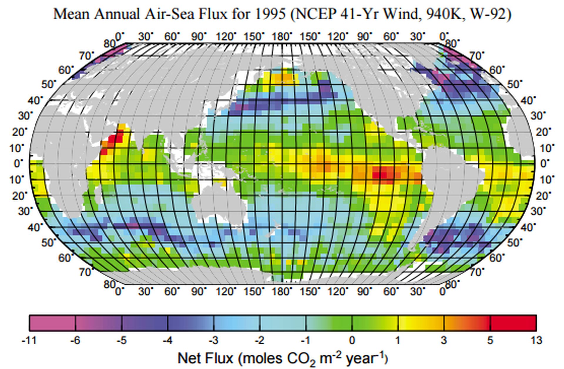
The lifetime of atmospheric CO2 results from its solubility in seawater, which solubility decreases with increasing temperature. A flow is established between the tropical oceans, which degas, and the mid-latitudes, which dissolve, benefiting from winds aloft.
The rapid equilibration of the isotopic composition of the atmosphere involves only the surface layer of the oceans and the biosphere (exchange of 13CO2 and 12CO2 molecules) while the sequestration of the atmospheric carbon dioxide occurs more in depth of the mixed layer of the oceans, carbonic acid being transformed into bicarbonates, then carbonates which precipitate.
Then, high contrast in durations of the impulse responses of 13CO2 and CO2 reflect the different mechanisms involved. Neither the biosphere nor the ocean surface permanently sequester atmospheric CO2, whether it produces biomass through photosynthesis as it is restored in the mineralization process after the death of plants (with the exception of alkanes formed in the deep ocean and fjords from phytoplankton as well as peat), or it is absorbed by the ocean surface due to degassing.
The enrichment of the atmosphere in anthropogenic CO2 comes from increasing emissions. Suppose that these emissions stabilize at the level of 2013. In this case, the increase in the concentration of anthropogenic CO2 would continue until 2043 to reach 150 ppmv. Beyond this date a steady state would occur, the CO2 emitted being transformed into carbonates and organic matter (alkanes, peat). Note that this limit value of 150 ppmv does not depend on the shape of the impulse response, but only of its area. It states that, in the event that the emissions would be stabilized in 2013, the concentration of anthropogenic CO2 in the atmosphere would be more than half that of the natural CO2 (atmospheric CO2 concentration was 285 ppmv in 1850). This increase in CO2 concentration of 150 ppmv would be below the cumulative emissions that would be 325 ppmv in 2043. Therefore, nearly half of the anthropogenic CO2 emitted since the beginning of the industrial era would have been sequestered.
Future changes in the concentration of atmospheric CO2 is easily established from the assumptions on anthropogenic emissions expressed in ppmv per year by accumulating the annual emissions over the last 30 years. Everything suggests that it will continue to increase at the present rate for many years, and this regardless of the policies to reduce emissions of greenhouse gases implemented by the various states.