The isotope analysis of ice cores plays a key role in understanding the different mechanisms involved in the natural evolution of climate over the last major cycles of glacial and interglacial periods. The oldest records obtained to date cover 800,000 years, the second half of the Quaternary. Deuterium data ²H obtained from Antarctica Dome C ice core (European Project for Ice Coring in Antarctica EPICA) are used for global mean temperature estimate in the southern hemisphere [Jouzel et al, 2007]. ¹⁸O data obtained from Greenland Summit Ice Cores GISP2 (Greenland Ice Sheet Project 2 Ice Core), Grootes and Stuiver, [1997] are used as proxies of global mean temperature in the northern Atlantic [Jouzel and Merlivat, 1984].

Contents

• • The natural variability of climate
  • However the solar irradiance variability has low direct impact on climate
  • A novel approach: the modulated response of subtropical gyres
  • The resonance of tropical waves
    • The tropical Atlantic Ocean
    • The tropical Pacific Ocean
    • The tropical Indian Ocean
  • The resonance of gyral Rossby waves
    • The short-period gyral Rossby waves
    • The long-period gyral Rossby waves
  • Where the earth is warming… or cooling
    • Baroclinic atmospheric instabilities
    • Rainfall oscillation: thermal exchanges between oceans and continents

    The natural variability of climate

    

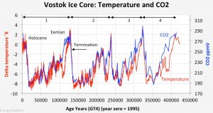
    From proxies derived from ice cores taken from the polar ice caps, the observed correlation between global surface temperature and atmospheric CO2 over the last four glacial-interglacial periods shows that it is the rise in temperature which increases the CO₂ in the atmosphere ( by degassing oceans mainly) and not the reverse, since the observed cycles are the result of orbital forcing (Milankovitch cycles).

    This process is still valid today but not noticeable yet because changing equilibriums of the mixed layer of the ocean requires several hundred years. By contrast the emission of combustion gases has a faster effect on the global temperature by radiative forcing.

    

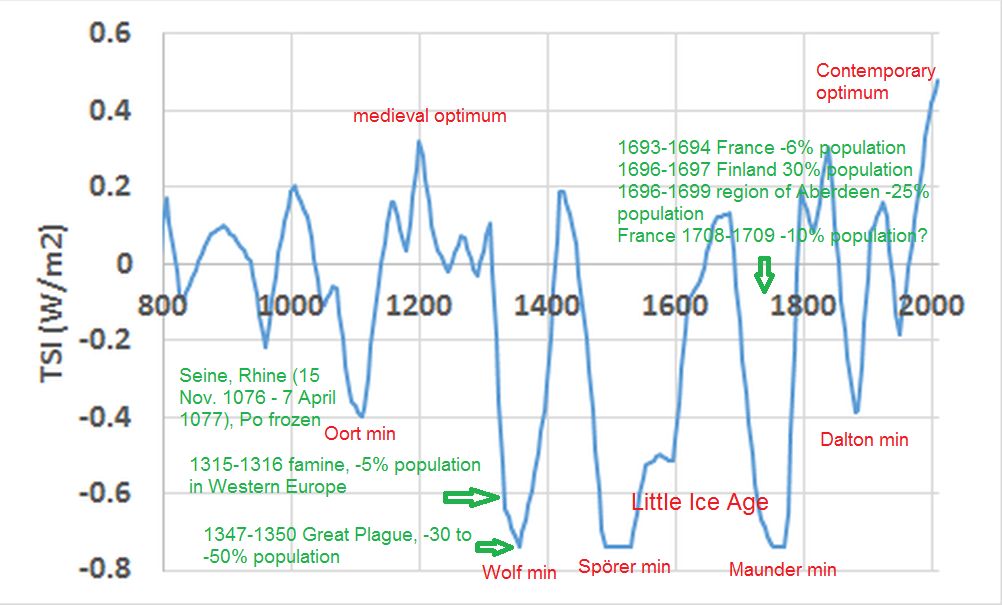
    Solar activity over the past 11,400 years has been reconstructed by analyzing jointly the concentration of radiocarbon in tree rings and isotopic abundance of beryllium-10 in ice cores. ¹⁴C and ¹⁰Be isotopes, which are produced by cosmic rays in the upper atmosphere, indeed reflect solar activity because in periods of high activity cosmic rays are deflected in the solar system and therefore produce less cosmogenic isotopes.

    The reconstruction of solar activity shows that it varies continuously. During the last millennium, humanitarian disasters generated during periods of low activity suggests that the global temperature has dropped, as was the case during the last Little Ice Age: there is undoubtedly a causal relationship between solar activity and global temperature.

    However the solar irradiance variability has low direct impact on climate

    How can the 11-year cycle, during which solar activity varies of a few tenths of a percent, be so quiet? Although low, this amplitude is of the same order as that of longer cycles. But this 11-year cycle has little influence on the climate compared to Milankovitch cycles, of very long-periods, which reflect the variations in the orbital parameters of the earth around the sun. Those have a significant impact, setting periods of glaciation, in particular. This selectivity and the variability in the efficiency of solar and orbital forcing during glacial-interglacial periods highlighted from the analysis of ice cores originating from Greenland and Antarctica suggest that resonance phenomena occur, filtering out some frequencies in favor of others while amplifying or mitigating according to the extension of the polar caps.

    A novel approach: the modulated response of subtropical gyres

    The direct impact of solar irradiance does not explain climate variability at different time scales. Such an assumption would come to imagine a submissive climatic system while it has its own frequencies, a considerable inertia, and manifests many whims, harbingers of resonant phenomena. The dynamics of climatic phenomena suggests a leading role of oceans whose influence, though long recognized, remains poorly understood. The oceans offer indeed a field of investigation whose scope is considerable, and that concerns the resonance of the oceanic planetary waves: it not only allows explaining and reproducing the warming of our planet, more precisely the middle and long-term climate variability, but also the El Niño phenomenon, the succession of wet or dry years observed in Western Europe since the 70’s…

    Is that the tropical belt of the oceans produces long-waves, whose wavelength is several thousand kilometers. Trapped by the equator due to the Coriolis force resulting from the earth’s rotation, they are deflected at the approach of the continents to form off-equatorial waves. These long tropical waves resonate with the forcing exerted by trade winds, whose period is annual, to produce sub-harmonic whose period is multi-annual. These long-waves that oceanographers appoint of the name of baroclinic result of the oscillation of the thermocline one hundred meters deep or more that separates the warm surface waters from deep cold waters, denser.

    This tropical oceanic resonance is one of the drivers of ocean surface circulation, i.e. above the thermocline, and contributes to the formation of strong western boundary currents such as the Gulf Stream in the North Atlantic and the Kuroshio in the northeast Pacific, by introducing a sequence of warm or cold waters according to the oscillation of the thermocline. Around latitude 40°N or S, those western boundary currents, which flow poleward in both hemispheres, leave the boundary of the continents to join each of the five oceanic subtropical gyres, giant vortexes at the north and south Atlantic and Pacific oceans and the southern Indian ocean. These resonantly forced baroclinic waves then become gyral, suiting their wavelength to the period inherited from the tropical oceans.

    For periods between half a year and eight years, the forcing of these gyral Rossby waves is induced from the sequence of warm and cold waters conveyed by western boundary currents, and now cause the oscillation of the thermocline of the gyre. But these gigantic gyral Rossby waves also have the ability to tune with the long-period solar cycles of one to up to several centuries, as well as Milankovitch cycles that affect the occurrence of glacial and interglacial periods, which reflect the changes in terrestrial astronomical parameters throughout tens of thousands of years.

    These resonant baroclinic waves have the ability to ‘hide’ the thermal energy that drives them by lowering the thermocline; due to a positive feedback those warm deep-waters favor the acceleration of the western boundary current and the development of sea surface temperature anomalies, supporting the heat exchanges between the ocean surface and the atmosphere: thermal surface anomalies induce atmospheric instabilities say again baroclinic, depressions or cyclones, which, carried by the jet-streams at high altitude, travel throughout the continents.

    In this way, surface temperature of continents respond to thermal anomalies of subtropical gyres. Positive or negative according to the motion of the thermocline, these thermal anomalies of sea surface, which result from the remanence of the vertical thermal gradient, tend to produce the same anomalies at the surface of continents. This because of the cyclonic or anticyclonic activity of the atmosphere stimulated at mid-latitudes. This thermal balancing internal to our planet, which occurs over the years, smooth the climate variations we observe daily at mid-latitudes. The imbalance between the energy received and re-emitted by the earth mainly depends on the depth of the thermocline of gyral Rossby waves.

    The resonance of tropical waves

    To understand the modulated response of subtropical gyres, driver of mid- and long-term climate variability and its coupling with the solar and orbital cycles, first we have to focus on the resonance of oceanic tropical waves from which are inherited periods of resonance. The study of the baroclinic quasi-stationary waves in the three tropical oceans consists in bringing out sea surface height anomalies and modulated currents in characteristic bands such as the 8-16 month band for annual waves. From measurements of sea surface height are deduced the amplitude and phase of sea surface height anomalies, but also the speed and phase of the modulated geostrophic currents from the slope of the sea surface, thanks to the use of cross wavelets.

    Quasi-Stationary-Waves are formed, representing a single dynamic phenomenon within a characteristic bandwidth. Geostrophic forces closely constrain the behavior of the baroclinic waves at the limits of the basin, forming antinodes at the place of Sea Surface Height anomalies and nodes where modulated geostrophic currents ensure the transfer of warm water from an antinode to another. Modulated geostrophic currents that change direction twice per cycle, are superimposed on the wind-driven current. Although these terms node and antinode are abusive because the phase of Quasi-Stationary-Waves is not uniform, which may involve overlapping of nodes and antinodes, they explicitly reflect the evolution of the wave during a cycle.

    The tropical Atlantic Ocean

    The tropical Atlantic Ocean is subject to the resonance of a quasi-stationary wave formed by an equatorial Kelvin wave and first baroclinic mode, first meridional mode equatorial and non-equatorial Rossby waves, forming a single dynamic system. This is tuned over the annual forcing period of the trade winds.

    The tropical Atlantic Ocean

    The tropical Pacific Ocean
    

    The tropical Pacific Ocean is subject to the resonance of two coupled dynamic systems, tuned over an annual and quadrennial period. The annual quasi-stationary wave is a first baroclinic mode, fourth meridional mode Rossby wave tuned over the annual period of forcing by the trade winds. The quasi-stationary quadrennial wave consists of an equatorial Kelvin wave and first baroclinic mode, first meridional mode equatorial and non-equatorial Rossby waves. The quadrennial wave is self-sustained by inducing an ENSO event at the end of its eastward phase propagation, while benefiting from the coupling with the annual quasi-stationary wave.

    The tropical Pacific Ocean

    The tropical Indian Ocean

    The tropical Indian Ocean is subject to the resonance of a quasi-stationary wave of semi-annual period formed by an equatorial Kelvin wave and first baroclinic mode, first meridional mode equatorial and non-equatorial Rossby waves. This quasi-stationary wave forms a single dynamic system forced by the monsoon winds. On the other hand, an annual non-equatorial wave originating in the Timor passage traverses the entire tropical Indian Ocean in each of the two hemispheres.

    The tropical Indian Ocean

    The resonance of gyral Rossby waves

    To the 5 subtropical gyres correspond 5 western boundary currents that are the Gulf Stream and the Brazil Current in the North and South Atlantic, the Kuroshio and the eastern Australian current in the North and South Pacific, the Agulhas in the South Indian Ocean. Under the influence of resonantly forced baroclinic waves, the three tropical oceans feed those western boundary currents through a sequence of warm and cold waters to one cycle every 1/2, 1, 4 and 8 years. Tropical oceans behave indeed as « resonators » under the effect of forcing due to surface stress and ENSO as regards the Pacific.

    In fact, during these cycles the temperature of the water carried by the western boundary currents does not change, or very little. The wavelet analysis of the sea surface temperature does not show anomalies in the different characteristic frequency bands. It is the depth of the thermocline that varies, thus the warm water mass transported poleward, without generating the formation of baroclinic waves that, facing west, would inevitably be wiped out against the coasts.

    This is no longer true when the western boundary current reaches a latitude nearby 35° to 40°N or S. At high latitudes, the velocity of the western boundary current increases as the phase velocity of the baroclinic waves decreases: baroclinic waves are formed when the velocity of the western boundary current becomes higher than their phase velocity.

    More precisely, the western boundary current becomes unstable when its speed is higher than the phase velocity of Rossby waves, this condition inducing a resonance. Any obstacle causing the current to move away from the coast leads to the formation of quasi-stationary Rossby waves, either because of the line of the coast or the collision with a current flowing in the opposite direction along the coast: the western boundary current orientates gradually eastwards while Rossby waves propagate in the opposite direction.

    Short-period Rossby waves

    Rossby waves form where the western boundary currents leave the continents to merge into each of the 5 subtropical gyres. Several coupled waves are superimposed, their wavelength being proportional to their periods locked in subharmonic mode.

    Short-period Rossby waves

    Long-period gyral Rossby waves

    Long period coupled gyral Rossby waves wrap around the 5 subtropical gyres. Propagating cyclonically, they are superimposed on the anticyclonic current of the gyre. In theory, the periods of long wavelength gyral Rossby waves have no upper limit. Their period being locked in subharmonic mode, the Rayleigh friction of these waves resonantly forced by the solar and orbital cycles is compensated by the lengthening of the duration of the forcing when the period increases.

    Long-period gyral Rossby waves

    Where the earth is warming… or cooling

    Baroclinic atmospheric instabilities

    The gyral and tropical resonance producing positive or negative surface temperature anomalies these can induce high and low atmospheric pressure systems that affect the climate globally. To quantify the energy transfer from the thermal anomaly to the continents, the unperturbed state of the system in the absence of thermal anomaly resulting from the resonance of baroclinic waves has to be considered at first, which implies that the average energy captured by the earth is completely re-emitted in space. This is only true if the energy transfers are averaged over one or even several years to remove fingerprints of phenomena not linked to the resonance of baroclinic waves, which cause an imbalance in energy budget during the annual cycle: this is the case, for example, of the formation of sea ice during the winter and its melting during the summer.

    Then, the perturbed state resulting from the imbalance in energy budget due to heat transfer toward high latitudes of the gyres behaves, which concerns ocean–atmosphere exchanges, like a quasi-isolated thermodynamic system. This is because thermal exchanges are mainly ruled by latent and sensible heat fluxes. Indeed, the difference in radiative fluxes between the surface of the gyres and that of the surrounding ocean is very low in comparison with other heat fluxes. This implies that the heat dissipated at the ocean–atmosphere interface at mid-latitudes is conserved on a planetary scale. Compared to the undisturbed system, the perturbed state of the system tends to a new steady state in which a new thermal equilibrium occurs between the sea surface perturbation ΔT and the continents. Due to its persistence, which reflects the renewal of the mixed layer at high latitudes of the gyres while maintaining the vertical temperature gradient, ΔT tends to balance with the surface temperature perturbation of the continents.

    Although the areas covered by oceanic thermal anomalies are small compared to the ocean surface, they generate atmospheric baroclinic instabilities that have a key role in the transfer of heat between the oceans and continents. However, the mechanisms involved differ depending on whether one considers the tropics or mid-latitudes. As we will see by referring to the rainfall oscillation in the band 5-10 years, thermal transfer, positive or negative, between the anomalies resulting from the resonance of baroclinic waves and impacted continental régions is performed in two main ways (Pinault, 2018a). On the one hand the oceanic temperature anomalies at mid-latitudes deflect tropical cyclones to mid-latitudes or otherwise confine them within the tropical belt according to the sign of the anomalies. On the other hand they promote depressions, anticyclones and troughs at mid-latitudes, these atmospheric phenomena being aroused under the effect of the polar or sub-tropical jet-stream. In all cases, atmospheric baroclinic instabilities may generate heat transfers to the synoptic scale, mainly in the form of latent heat.

    Rainfall oscillation: thermal exchanges between oceans and continents

    To highlight how some land areas are affected by atmospheric baroclinic instabilities induced by thermal anomalies resulting from the resonance of baroclinic waves, it is convenient to use monthly rainfall height data which are known since 1901 on the terrestrial scale. Indeed, heat transfer from the oceans to the continents mainly resulting from processes of evaporation and condensation according to what has been seen previously, how rainfall varies over time characterizes the impacted areas.

    Rainfall oscillation

    Glossary

    Dansgaard–Oeschger events (often abbreviated D–O events) are rapid climate fluctuations that occurred during the last glacial period.

    The term stable isotopes usually refers to isotopes of the same element. The relative abundance of such stable isotopes can be measured experimentally (isotope analysis), yielding an isotope ratio: relative abundances are affected by isotope fractionation in nature, hence their interest in geochemistry.

    In meteorology, synoptic scale phenomena are characterized by a length of several hundred to several thousand kilometers and a period of several days.

    A standing wave is the phenomenon resulting from the simultaneous propagation in different directions of several waves of the same frequency. In a standing wave nodes remain fixed, alternating with antinodes. A quasi-stationary wave acts as a standing wave but the antinodes and nodes may overlap.

    Geostrophic currents are derived from measurements of wind, temperature and satellite altimetry. The calculation uses a quasi-stationary geostrophic model while incorporating a wind-driven component resulting from wind stress. Geostrophic current thus obtained is averaged over the first 30 meters of the ocean.

    The Coriolis parameter f is equal to twice the speed of rotation Ω of the earth multiplied by the sine of the latitude φ: f = 2Ωsin φ. The Coriolis force, on the other hand, is perpendicular to the direction of movement of the moving body. It is proportional to the velocity of the body and the speed of rotation of the medium.

    Baroclinic wave. In contrast with barotropic waves that move parallel to isotherms, baroclinic Rossby or Kelvin waves cause a vertical displacement of the thermocline, often of the order of several tens of meters. The seconds are usually slower than the first.

    Jet-streams are fast winds aloft blowing from west to east. Along a curved and sinuous path, they play a major role in atmospheric circulation as they participate in the formation of depressions and anticyclones at middle latitudes, which then move under these powerful atmospheric currents.

    Baroclinic instability draws energy from the portion of the potential energy available to be converted. Available potential energy is dependent upon a horizontal gradient of temperature. The conversions of energy are proportional to perturbation heat fluxes in the horizontal and vertical that, as part of this article, are related to oceanic thermal anomalies resulting from the resonance of baroclinic waves. A horizontal temperature gradient implies the presence of vertical shear. So, baroclinic instability is also an instability of the vertical shear.

    Western boundary currents, warm, deep, narrow and fast are formed along the western boundary of the ocean. They carry warm water from the tropics to the poles, forming the western branch of the subtropical gyres. It is the Gulf Stream (North Atlantic), the Brazil Current (South Atlantic) the Agulhas (South Indian Ocean), the Kuroshio (North Pacific), and the western boundary currents of the subtropical gyre in the South Pacific.

    Positive feedback loops amplify changes in a dynamic system; this tends to move the system away from its equilibrium state and make it more unstable. Negative feedbacks tend to dampen changes; this tends to hold the system to some equilibrium state making it more stable.

    The adiabatic lapse rate is, in the Earth’s atmosphere, the variation of air temperature with altitude (in other words, the gradient of the air temperature). Adiabatic means that a mass of air does not exchange heat with its environment (other air masses, relief). If we exclude condensation (formation of clouds and precipitation) and vaporization, the lapse rate of the atmosphere depends only on the pressure.